RNA-seq and differential expression power analysis

Overview

A reader requested a detailed protocol for the Methods of our paper section titled “RNA-seq and differential expression power analysis”. This section details how we aligned RNA-seq reads for human and chimp samples, performed differential expression (DE) testing, and performed an extensive power analysis by sub-sampling varying numbers of individuals to include in the DE testing. The results of this section are summarized in Fig1 and its associated supplemental figures. In summary,

• We generated RNA-seq data for 39 chimpanzee post-mortem heart tissue samples, 10 human samples, and utilized publicly available GTEx data for additional human samples.
• Chimp RNA-seq samples and human samples easily separate, except for a few outlier samples which we excluded from further analysis
• With our relatively large sample size of DE testing, we identify thousands of differentially expressed genes, the exact number of course depends on the level of statistical stringency to call something “differentially expressed”.
• We utilized our relatively large sample size to subsampled small sample sizes to better understand how sample size and sequencing depth effects DE results. We find that
  • Samples sizes influences number of DE genes moreso than sequencing depth.
  • Using the full dataset as the “true” set of DE genes, we find that FDR is generally well calibrated at smaller sample sizes
  • Note that the quantitative results of this power analysis may not extrapolate perfectly to comparisons in different species or tissues. Obviously more divergent species comparisons will probably have more differentially expressed genes than human vs chimp, all else being equal.

Here I will provide more detials of the analysis steps for this section First, some notes on raw data and code availability:

• Publicly available raw data for this publication is described here,
• all code associated with this paper is in this git repository (but I make no promises on the cleanliness of my code!). This contains code that I used to go from raw data to partially processed and final figures displayed in the publication.
• Additionally, nitty details and R code for some of data exploration can be found on the website associated with that repo.

Here is the “RNA-seq and differential expression power analysis” methods section, copied verbatim from the publication:

39 RNA-seq fastq files for human left ventricle were chosen at random from GTEx v7 (Figure 1—source data 1, see Acknowledgements). Additionally, the 10 human and 18 chimpanzee RNA-seq libraries previously generated (Pavlovic et al., 2018), and all the novel chimpanzee RNA-seq libraries generated in this study are described in Figure 1—source data 1. Fastq files for samples that were sequenced on multiple lanes were combined after confirmation that all gene expression profiles for all fastq files cluster primarily by sample and not by sequencing lane. GTEx-derived fastq files were trimmed to 75 bp single-end reads to match the non-GTEx sequencing data. Reads were aligned to the appropriate annotated genome (GRCh38.p13 or Pan_tro_3.0 from Ensembl release 95; Zerbino et al., 2018) using STAR aligner (Dobin et al., 2013) default parameters. Only chromosomal contigs were considered for read alignment throughout this work. That is, unplaced contigs were excluded from the reference genome. Gene counts were obtained with subread featureCounts (Liao et al., 2014) using a previously described annotation file of human-chimpanzee orthologous exons (Pavlovic et al., 2018).

So far, the steps described include downloading fastq reads, aligning them to the genome with STAR, and counting reads per gene are standard analysis steps which I will not detail here, though my code for doing so is available in the git repo as part of a giant Snakemake pipeline, see this part of the pipeline for most of the relevant code for entire section. Additionally, here is one of many tutorials I found online for these steps. Next, I describe how we did differential expression (DE) testing and a power analysis to better understand how sample size and read depth effect our chimp-human DE test results:

The gene expression matrix was converted to CountsPerMillion (CPM) with edgeR (Robinson et al., 2010) to normalize reads to library size. The mean-variance trend was estimated using limma-voom (Ritchie et al., 2015). Genes with less than 6 CPM in all samples were excluded from further analysis. This cutoff was chosen based on visual inspection of the voom mean-variance trend to identify where the trend becomes unstable. To normalize differences in orthologous exonic gene size between human and chimpanzee, we converted the log(CPM) matrix to log(RPKM) based on the species-specific length of orthologous exonic regions. We then visually inspected PCA plots and hierarchical clustering to identify potential outliers and batch effects (Figure 1). We note that although all the chimpanzee RNA isolation and sequencing were prepared separately from GTEx heart samples, PCA and clustering analysis suggest that the inter-species differences vastly outweigh the technical batch effects (based on the inter-species but within-batch samples sourced from Pavlovic et al., 2018). The dataset of 49 human samples and 39 chimpanzee samples was culled to 39 human and 39 chimpanzee samples based on exclusion of 5 obvious human outliers which did not cluster with the rest and had among the lowest read depths (Figure 1A–B). The remaining human samples to exclude to reach a balanced set of 39 human and 39 chimpanzee samples were chosen by excluding the remaining GTEx samples with the lowest mapped read depths. Differential expression was tested using limma (Ritchie et al., 2015), using the eBayes function with default parameters and applying Benjamini-Hochberg FDR estimation. For Figure 1—figure supplement 2, this process was repeated at varying sample size (sampling with replacement) and at various read depths. Sequencing depth subsampling analysis was performed at the level of bam files to obtain matched numbers of mapped reads across samples and differential expression analyses was repeated.

• Firstly note I think there is a typo, though I don’t think it would change any of the main conclusions: Sampling smaller sizes was done without replacement… It makes little sense I think to sample with replacement for a DE analysis where the presence of identical samples violates lots of model assumptions. Anyway, in the rest of this document, I will detail how these steps were performed in R… I start from the output of featureCounts, which is tracked in the git repo.

Setup

First, let’s load all the necessary libraries and print session info so that our R environment can be reproduced:

library(tidyverse)
library(limma)
library(edgeR)
library(gplots)
library(pROC)

sessionInfo()

## R version 3.6.1 (2019-07-05)
## Platform: x86_64-apple-darwin15.6.0 (64-bit)
## Running under: macOS Catalina 10.15.7
## 
## Matrix products: default
## BLAS:  /Library/Frameworks/R.framework/Versions/3.6/Resources/lib/libRblas.0.dylib
## LAPACK: /Library/Frameworks/R.framework/Versions/3.6/Resources/lib/libRlapack.dylib
## 
## locale:
## [1] en_US.UTF-8/en_US.UTF-8/en_US.UTF-8/C/en_US.UTF-8/en_US.UTF-8
## 
## attached base packages:
## [1] stats    graphics  grDevices utils     datasets methods   base     
## 
## other attached packages:
##  [1] pROC_1.15.3     gplots_3.0.1.1  edgeR_3.26.8    limma_3.40.6   
##  [5] forcats_0.4.0   stringr_1.4.0   dplyr_1.0.2     purrr_0.3.3    
##  [9] readr_1.3.1     tidyr_1.0.0     tibble_3.0.3    ggplot2_3.3.2  
## [13] tidyverse_1.3.0
## 
## loaded via a namespace (and not attached):
##  [1] Rcpp_1.0.5         locfit_1.5-9.1     lubridate_1.7.9    lattice_0.20-38   
##  [5] gtools_3.8.1       assertthat_0.2.1   digest_0.6.27      R6_2.4.1          
##  [9] cellranger_1.1.0   plyr_1.8.6         backports_1.1.5    reprex_0.3.0      
## [13] evaluate_0.14      httr_1.4.1         pillar_1.4.6       rlang_0.4.7       
## [17] readxl_1.3.1       rstudioapi_0.10    gdata_2.18.0       rmarkdown_1.18    
## [21] munsell_0.5.0      broom_0.7.0        compiler_3.6.1     modelr_0.1.5      
## [25] xfun_0.11          pkgconfig_2.0.3    htmltools_0.4.0    tidyselect_1.1.0  
## [29] fansi_0.4.0        crayon_1.3.4       dbplyr_1.4.2       withr_2.1.2       
## [33] bitops_1.0-6       grid_3.6.1         jsonlite_1.6       gtable_0.3.0      
## [37] lifecycle_0.2.0    DBI_1.0.0          magrittr_1.5       scales_1.1.1      
## [41] KernSmooth_2.23-16 cli_2.0.0          stringi_1.4.3      fs_1.3.1          
## [45] xml2_1.2.2         ellipsis_0.3.0     generics_0.0.2     vctrs_0.3.4       
## [49] tools_3.6.1        glue_1.4.2         hms_0.5.2          yaml_2.2.0        
## [53] colorspace_2.0-0   caTools_1.17.1.3   rvest_0.3.5        knitr_1.26        
## [57] haven_2.2.0

Next, let’s load the gene expression count table for the full dataset of all RNA-seq samples used in this publication. This data is tracked in the git repository. Technically, one could download the raw sequencing data for this publication then use code in the git repository to recreate this data. But that requires aligning lots of reads and using featureCounts to create the gene expression count table (genes as rows, samples as columns, each cell is read count), which is all very computationally intensive. So here we will just use the gene expression count table that I have pre-processed in this repository.

Reading in the data

#Clone the git repo to a temporary directory so as to not clash with any pre-existing files.
RepoPath <- paste0(tempdir(), "/Comparative_eQTL")
cmd <- paste("git clone --depth 1 https://github.com/bfairkun/Comparative_eQTL.git", RepoPath)
system(cmd)

#Read in the featureCounts output. I have a featureCounts output file for chimp samples and a separate one for humans.
CountTableChimpFile <- paste0(tempdir(), "/Comparative_eQTL/output/PowerAnalysisFullCountTable.Chimp.subread.txt.gz")
CountTableHumanFile <- paste0(tempdir(), "/Comparative_eQTL/output/PowerAnalysisFullCountTable.Human.subread.txt.gz")

CountTableChimp <- read_delim(CountTableChimpFile, delim='\t', skip = 1)
CountTableHuman <- read_delim(CountTableHumanFile, delim='\t', skip = 1)

#Merge all human and chimp count tables into one giant count table.
CombinedTable <- inner_join(CountTableChimp[,c(1,7:length(CountTableChimp))], CountTableHuman[,c(1,7:length(CountTableHuman))], by=c("Geneid")) %>%
  column_to_rownames("Geneid") %>% as.matrix()

#Preview a little bit of the CombinedTable count table
CombinedTable[1:5,1:5]

##                                     4x0519  4x373  476  4x0025  438
## ENSG00000273443      0           0          0      4           0
## ENSG00000217801      8           3          1      6           2
## ENSG00000237330      3           0          2      0           0
## ENSG00000223823      0           0          0      0           0
## ENSG00000207730      0           1          0      0           0

#Check the column (sample) names
colnames(CombinedTable)

##  [1] "4x0519"      "4x373"      "476"          "4x0025"     "438"       
##  [6] "462"           "4X0354"    "503"          "317"           "623"       
## [11] "554"          "4X0095"    "549"          "4X0267"     "4X0339"    
## [16] "529"          "495"          "338"          "4X0550"     "558"       
## [21] "4x523"      "389"          "4x0043"     "4X0357"     "88A020"    
## [26] "554_2"      "Little_R"     "676"           "456"           "537"       
## [31] "MD_And"  "724"          "4x0430"     "95A014"     "4X0333"    
## [36] "522"          "295"          "4X0212"     "570"           "SRR1477033"
## [41] "SRR598148"    "SRR601645"  "SRR599086"       "SRR604230"     "SRR1478149"
## [46] "SRR1478900"  "SRR598509"  "SRR1478189"     "SRR613186"     "59263"     
## [51] "SRR1477015"  "62905"          "63060"                "SRR600852"     "62606"     
## [56] "SRR601986"    "SRR604174"  "SRR608096"       "SRR1489693"   "62765"     
## [61] "61317"            "59167"           "SRR614996"       "SRR602106"     "SRR1507229"
## [66] "SRR601868"    "SRR612335"  "SRR598589"       "SRR600474"     "SRR603449" 
## [71] "SRR606939"    "SRR1481012" "SRR599249"       "59365"            "SRR607313" 
## [76] "63145"            "SRR603918"  "SRR1474730"      "SRR1477569"  "SRR601239" 
## [81] "SRR607252"    "SRR612875"  "SRR601613"        "SRR614683"    "SRR604122" 
## [86] "59511"            "62850"          "SRR599380"

Note that the input here has some sample labels which are based on the SRR accession numbers from when I downloaded the raw data from GTEx. For publication in Fig1A-C, I used GTEx individual identifiers to label the GTEx samples rather than SRR accession numbers. So let’s convert those sample identifiers to their GTEx identifier. Sample information is in Fig1-SourceData1

#Read in Fig1-SourceData1
SampleMetaInfo <- read.table(url("https://cdn.elifesciences.org/articles/59929/elife-59929-fig1-data1-v2.txt"), sep='\t', header=T, stringsAsFactors = F) %>%
  #And add a column that should match the CountTable SampleName
  mutate(ID_in_CountTable = case_when(
    is.na(SRA) ~ Sample.ID,
    TRUE ~ SRA
  )) %>%
  #And given the samples a new name, by conatenating the Sample.ID and Species columns
  mutate(NewName = paste0(Sample.ID, ".", SP))
  
head(SampleMetaInfo)

##   Sample.ID Alternate.ID RNA.Extraction.Batch RIN SX Age Post.mortem.time.min
## 1      295          Duncan             10/10/18 7.3  M  40                   30
## 2      317          Iyk                     6/7/16 7.6  M  44                      150
## 3      338          Maxine              6/7/16 7.2  F  53                        NA
## 4      389          Rogger             10/10/18 5.7  M  45                   NA
## 5      438          Cheeta              6/22/16 5.6  F  55                      NA
## 6      456          Mai                    6/22/16 5.5  F 49                      NA
##                                     TissueSource Notes    SP  SRA
## 1                                         Yerkes  <NA> Chimp <NA>
## 2 Yerkes; Library from Pavlovic et al resequenced  <NA> Chimp <NA>
## 3 Yerkes; Library from Pavlovic et al resequenced  <NA> Chimp <NA>
## 4                                         Yerkes  <NA> Chimp <NA>
## 5 Yerkes; Library from Pavlovic et al resequenced  <NA> Chimp <NA>
## 6 Yerkes; Library from Pavlovic et al resequenced  <NA> Chimp <NA>
##  PercentUniquelyMappingReads UniquelyMappingReads ID_in_CountTable   NewName
## 1                       85.77            155290675              295 295.Chimp
## 2                       82.74             68092789              317 317.Chimp
## 3                       83.70             80065396              338 338.Chimp
## 4                       86.35             99251068              389 389.Chimp
## 5                       82.43             77548087              438 438.Chimp
## 6                       84.28             88729841              456 456.Chimp

#Now rename the samples in the CountTable according to the Species and Sample.ID in SampleMetaInfo
#First, get named vector to translate CountTable colnames to new colnames
NamedVector <- SampleMetaInfo %>%
  dplyr::select(NewName, ID_in_CountTable) %>%
  deframe()

#Rename the columns of the CombinedTable
CombinedTable <- CombinedTable %>%
  as.data.frame() %>%
  rename(!!! NamedVector) %>%
  as.matrix()

Basic Quality-control

Ok. So now that we have the gene expression count table, let’s plot some basic quality control things…

#Plot depth per sample, This is basically Fig1A.
CombinedTable %>% colSums() %>% as.data.frame() %>%
  rownames_to_column("Sample") %>%
  mutate(Species=str_replace(Sample, ".+\\.(.+$)", "\\1")) %>%
  ggplot(aes(x=Sample, y=., fill=Species)) +
  geom_col() +
  scale_y_continuous(expand = c(0, 0)) +
  facet_grid(~Species, scale="free") +
  theme_bw() +
  ylab("Total gene-mapped read counts") +
  theme(axis.text.x = element_text(angle = 90, hjust = 1, size=6))

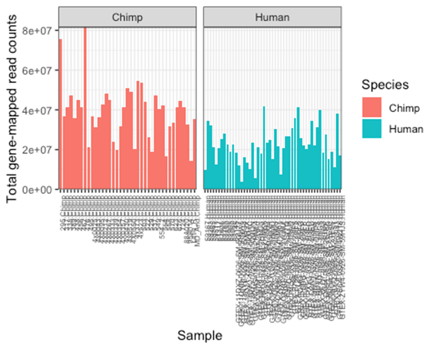
Notice there are a couple samples with really low read depth (total counts). Particularly in the human side. 10 of the human samples were from (Pavlovic et al), and the others were randomly chosen from GTEx. As described in the Methods section of the paper, I purposefully downloaded extra human samples anticipating that we should drop some from our analysis because they wouldn’t be high quality in some aspects.

Now let’s plot correlation matrix of gene expression values. This is one additional way to find outlier samples. You could consider filtering out lowly expressed genes before making this correlation matrix, but here I will just plot correlation matrix without filtering, since I am just using this to further justify throwing out the samples with low read depth.

#Use edgeR cpm function to calculate CountsPerMillion expression matrix.
cpm <- cpm(CombinedTable, log=TRUE, prior.count=0.5)
cpm[1:5,1:5]

##                 4x0519.Chimp 4x373.Chimp 476.Chimp 4x0025.Chimp 438.Chimp
## ENSG00000273443    -5.898265  -5.898265 -5.898265    -2.987845 -5.898265
## ENSG00000217801    -2.526536  -2.606798 -5.106758    -2.468307 -3.779182
## ENSG00000237330    -3.726191  -5.898265 -4.598574    -5.898265 -5.898265
## ENSG00000223823    -5.898265  -5.898265 -5.898265    -5.898265 -5.898265
## ENSG00000207730    -5.898265  -3.923604 -5.898265    -5.898265 -5.898265

#Create a vector to color the columns in the correlation matrix heatmap 
SpeciesFactor <- colnames(cpm) %>% endsWith("Human") %>% factor() %>% unclass() %>% as.character()

# Spearman correlation matrix heatmap. This is quite similar to Fig1B
cor(cpm, method = c("spearman")) %>%
heatmap.2(trace="none", ColSideColors=SpeciesFactor)

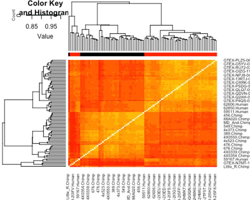
I notice that samples mostly cluster by species. This is to be expected. But there are a handful of samples that did not cluster in this way (the cluster on the lower left), and looking at the sample labels, I noticed they are mostly all the low read depth samples which I plotted above. I therefore felt justified further excluding human samples from further analysis mostly on the basis of low read depth. In detail (and as described in the Methods section of the paper), I removed all of the human samples in the lower left which did not cluster as expected. Almost all of these samples had amongst the lowest read depth (See Fig1A-B). I further removed human samples by lowest read depth until we were left with a set of 39 human and 39 chimp samples to do DE analysis on. This information on what samples I dropped are plotted in Fig1, and I am now noticing they are also implicitly in Fig1-SourceData1 if they have NA in the UniquelyMappingReads column. Let’s just drop those samples from further analysis now based on that column…

#Create a character vector of samples to drop based on presence of NA in UniquelyMappingReads column
SamplesToDrop <- SampleMetaInfo %>%
  filter(is.na(UniquelyMappingReads)) %>%
  pull(NewName)
  
#Drop the samples from the count table
CombinedTable <- CombinedTable %>%
  as.data.frame() %>%
  dplyr::select(-SamplesToDrop) %>%
  as.matrix()

Ok. Now let’s continue with some more QC before doing any DE testing. The next thing often done is to filter out lowly expressed genes. There are many reasonable methods for doing this. Usually people turn out leaving 10,000 - 15,000 genes for DE analysis, since the other genes tend to be too lowly expressed in any given cell/tissue type to make reliable inferences about.

#Make edgeR DGEList object from the count table, since edgeR has convenient functions to calculate cpm which we can use later.
d0 <- DGEList(CombinedTable)

#Calculate normalization factors before filtering lowly expressed genes
d0 <- calcNormFactors(d0)

#Chose some criteria to filter out lowly expressed genes. Here we chose to filter out genes in which the max expression value across all samples was less than 6 CountsPerMillion (cpm).
cutoff <- 6
drop <- which(apply(cpm(d0), 1, max) < cutoff)
d <- d0[-drop,]

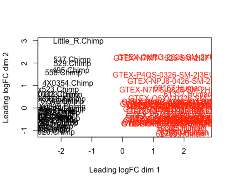
#limma has a plotMDS function, which should be basically the same thing as the PCA I plotted in Fig1C.
SpeciesFactor <- colnames(d) %>% endsWith("Human") %>% factor() %>% unclass() %>% as.character()
plotMDS(d, col = as.numeric(SpeciesFactor))

#What are the dimensions of this filtered expression matrix
dim(d)

## [1] 13604    78

As expected, all samples clearly cluster by species after…So in summary, our criteria for dropping out low quality samples, and filtering out lowly expressed genes, left us a count table with 13488 expressed genes, across 78 samples (39Human + 39Chimp). Now we can do DE testing

DE testing

We used voom and limma to do DE testing, using a linear model to test for effect of species on logRPKM. There are many other detailed tutorials online on doing things like this with RNA-seq data. Here is a tutorial that uses similar detailed methods as here. Some other packages for RNA-seq analysis use count based models (eg negative binomial model) to test for differential expression. However, in our cross-species analysis, we want to account for interspecies differences in gene length as a technical factor. This can in theory also be addressed in a count based model, but might be more simply addressed by a model that first normalizes the response variable by gene length (in other words, modeling rpkm instead of cpm), and then using non-count based models. Our lab has used this limma-voom interspecies DE approach in previous publications as well, for example Pavlovic et al. Also see Law et al

#First create a model matrix to define what factors to model. One could consider adding things like batch as covariates. I only included one term for species here.
mm <- model.matrix(~0 + SpeciesFactor)

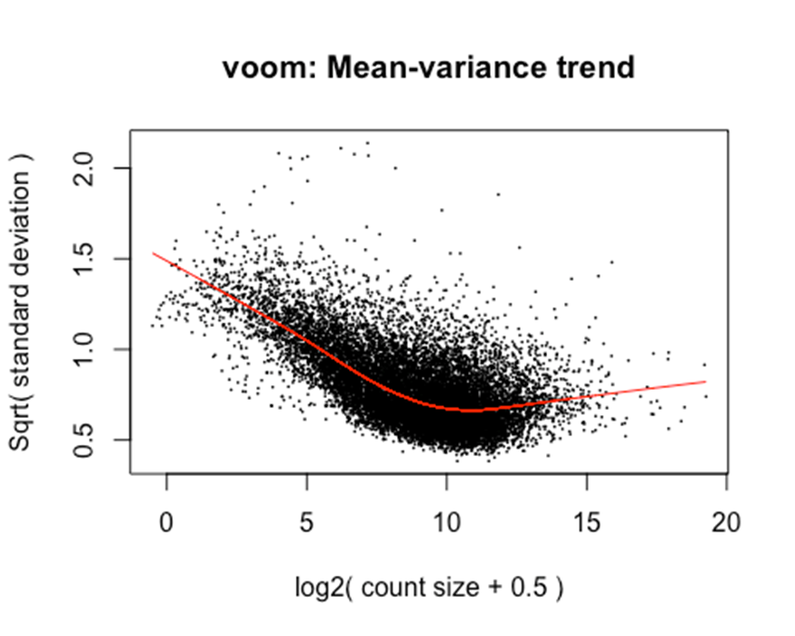
#Voom calculates CountsPerMillion (cpm) and also estimates empirical mean-variance trend to pass to limma
y <- voom(d, mm, normalize.method="cyclicloess", plot=T)

#Preview the logCPM matrix that voom outputs
y$E[0:10,0:10]

##                 4x0519.Chimp 4x373.Chimp  476.Chimp 4x0025.Chimp 438.Chimp
## ENSG00000186891  0.007264354   2.192026 -0.9730239   -0.2026754 -1.863854
## ENSG00000186827  2.318082750   4.545849  2.3616850    3.3906006 2.689233
## ENSG00000078808  6.810600319   6.600925  6.5768034    6.6654651 6.402233
## ENSG00000176022  4.355740832   4.489791  4.5035405    5.0603767 5.010610
## ENSG00000184163 -2.772817424    1.545452 1.2331913    0.7937947  1.526390
## ENSG00000160087  3.818533050   4.005223  4.0824893    4.2813741 4.013468
## ENSG00000162572 -2.775482002   -1.915168 -1.4715472   -3.8521053 -1.990108
## ENSG00000131584  5.612555496   6.301077  5.5557021    6.0360392 5.707724
## ENSG00000169972  2.359039307   2.220282  2.6958969    2.7626247 2.957855
## ENSG00000127054  5.828671663   6.678564  6.5648217    6.4146347 6.726868
##                  462.Chimp 4X0354.Chimp  503.Chimp 317.Chimp  623.Chimp
## ENSG00000186891 -1.2250263     1.727711 -0.6854836 -1.4178264 -2.5171085
## ENSG00000186827  1.6174419    5.176544  2.4816963  2.9908840 1.4075419
## ENSG00000078808  6.5156999    5.938869  6.8292671  6.8233637 6.7587739
## ENSG00000176022  4.8790983    4.063219  4.5669684  4.2743804 4.2947440
## ENSG00000184163 -0.3052323     1.850811 1.3801238 -0.5183195 -0.5084478
## ENSG00000160087  3.8540865    3.438767  4.3412314  3.8204245 4.2124553
## ENSG00000162572 -1.1500294    -1.304063 -1.4755990 -1.8888314 -1.3341264
## ENSG00000131584  5.0088610    7.818638  5.4870227  5.2940221 5.7967302
## ENSG00000169972  2.7519823    2.050862  2.5201906  1.8700041 2.9846884
## ENSG00000127054  5.6717842    7.295218  6.4448515  6.1769861 6.5259728

#Note that voom also outputs precision weights to account for mean variance trend when fitting a model
 

y$weights[0:10, 0:10]

##            [,1]      [,2]     [,3]      [,4]      [,5]     [,6]      [,7]
##  [1,] 1.0152616 0.6002381 1.1770889 0.8517961 0.7522019 0.8873568 0.7002918
##  [2,] 3.4888462 1.9973637 3.8992596 2.9944390 2.6377820 3.1095878 2.4307265
##  [3,] 4.4757778 5.1523261 4.2837682 4.7209896 4.9080570 4.6617417 5.0132583
##  [4,] 4.9491062 3.5827562 5.0992345 4.6600575 4.3503904 4.7382298 4.1272074
##  [5,] 1.5513607 0.8444988 1.8110608 1.2768479 1.1045336 1.3378315 1.0146684
##  [6,] 4.6682368 3.0931886 4.9058105 4.2484987 3.8594355 4.3613107 3.6212517
##  [7,] 0.5718497 0.3727787 0.6399482 0.4991060 0.4516049 0.5154511 0.4256014
##  [8,] 4.8376680 5.0262580 4.6427419 5.0616862 5.1511111 5.0162225 5.1531421
##  [9,] 3.0016072 1.6479295 3.3915805 2.5352186 2.2050896 2.6442570 2.0217405
## [10,] 4.5534406 5.1577820 4.3604826 4.7999446 4.9813366 4.7401198 5.0734769
##           [,8]      [,9]     [,10]
##  [1,] 0.9320520 0.8488373 0.7730581
##  [2,] 3.2480681 2.9848217 2.7175147
##  [3,] 4.5928885 4.7260537 4.8657289
##  [4,] 4.8248487 4.6534341 4.4282619
##  [5,] 1.4132991 1.2717598 1.1407959
##  [6,] 4.4903154 4.2380018 3.9478555
##  [7,] 0.5354956 0.4977357 0.4618158
##  [8,] 4.9522173 5.0656059 5.1440418
##  [9,] 2.7765241 2.5257125 2.2764262
## [10,] 4.6706859 4.8050442 4.9418406

The mean variance trend learned from voom uses log(cpm). However, note that we actually want to estimate gene expression between species, which we will express as log(rpkm) since the exonic gene length between human and chimp varies slightly for some genes. As per the voom publication Law et al 2014 log-cpm values output by voom can be converted to log-rpkm by subtracting the log2 gene length in kilobases. To accomplish this in R, I will make a matrix of gene lengths based on chimp orthologous exon length and human orthologous exon lengths to subtract the correct length for each species from the logCPM matrix output by voom. We can grab the exonic gene lengths from the featureCounts output.

#Create data frame storing gene lengths
GeneLengths <- inner_join(CountTableChimp[,c("Geneid", "Length")], CountTableHuman[,c("Geneid", "Length")], by=c("Geneid"), suffix=c(".Chimp", ".Human")) %>%
  right_join(
    data.frame(Geneid = rownames(y$E)),
    by="Geneid")

head(GeneLengths)

## # A tibble: 6 x 3
##  Geneid          Length.Chimp Length.Human
##  <chr>                 <dbl>        <dbl>
## 1 ENSG00000186891         1363         1370
## 2 ENSG00000186827         1565         1565
## 3 ENSG00000078808         3750         3764
## 4 ENSG00000176022         2761         2777
## 5 ENSG00000184163         1791         1794
## 6 ENSG00000160087         3082         3085

#Create a matrix with gene lengths that is the same dimensions as y$E, so that we easily subtract the gene lengths to arrive at logRPKM instead of logCPM
GeneLengths.mat <- matrix(data=NA, nrow(y$E), ncol(y$E))
for (i in 1:ncol(y$E)){
  Species <- gsub(".+\\.(.+?)$", "\\1",colnames(y$E)[i])
  if (Species == "Human"){
   GeneLengths.mat[,i] <- GeneLengths$Length.Human
  } else if (Species == "Chimp"){
   GeneLengths.mat[,i] <- GeneLengths$Length.Chimp
  }
}

#Preview the gene lengths matrix
GeneLengths.mat[0:10, 0:10]

##       [,1] [,2] [,3] [,4] [,5] [,6] [,7] [,8] [,9] [,10]
##  [1,] 1363 1363 1363 1363 1363 1363 1363 1363 1363 1363
##  [2,] 1565 1565 1565 1565 1565 1565 1565 1565 1565 1565
##  [3,] 3750 3750 3750 3750 3750 3750 3750 3750 3750 3750
##  [4,] 2761 2761 2761 2761 2761 2761 2761 2761 2761 2761
##  [5,] 1791 1791 1791 1791 1791 1791 1791 1791 1791 1791
##  [6,] 3082 3082 3082 3082 3082 3082 3082 3082 3082 3082
##  [7,] 4004 4004 4004 4004 4004 4004 4004 4004 4004 4004
##  [8,] 5621 5621 5621 5621 5621 5621 5621 5621 5621 5621
##  [9,] 1199 1199 1199 1199 1199 1199 1199 1199 1199 1199
## [10,] 3645 3645 3645 3645 3645 3645 3645 3645 3645  3645

#Reassign the voom expression matrix to convert from logCPM to logRPKM
y$E <- y$E - log2(GeneLengths.mat/1000)

Ok, now we are ready to do DE testing…

#fit linear model
fit<- lmFit(y, mm)

#define contrasts
contr <- makeContrasts(DE=SpeciesFactor1-SpeciesFactor2, levels = mm)

#fit contrasts
tmp <- contrasts.fit(fit, contrasts=contr)

#compute test statistics, pvals
efit <- treat(tmp, lfc = 0)

#topTable function presents all the results as a nice dataframe, included FDR adjusted P.vals
Results <- topTable(efit, n=Inf, sort.by="none")
head(Results)

##                      logFC    AveExpr         t     P.Value    adj.P.Val
## ENSG00000186891  2.7047227 -1.9403275  7.407938 1.136318e-10 7.223585e-10
## ENSG00000186827  0.6927307 1.9361685  2.761243 7.133880e-03 1.237716e-02
## ENSG00000078808 -0.2962773  5.0745793 -3.812835 2.682939e-04 6.040831e-04
## ENSG00000176022  0.1434711 2.9844008  1.848176 6.825921e-02 9.629766e-02
## ENSG00000184163  0.6198209 -0.2937247  2.580381 1.169069e-02 1.945921e-02
## ENSG00000160087 -0.1630316  2.5362072 -2.325832 2.255160e-02 3.532541e-02

#Plot volcano plot. Basically FigS1A
ggplot(Results, aes(x=logFC, y=adj.P.Val)) +
  geom_point(alpha=0.1) +
  scale_y_reverse() +
  scale_y_continuous(trans="log10") +
  ylab("FDR") +
  theme_bw()

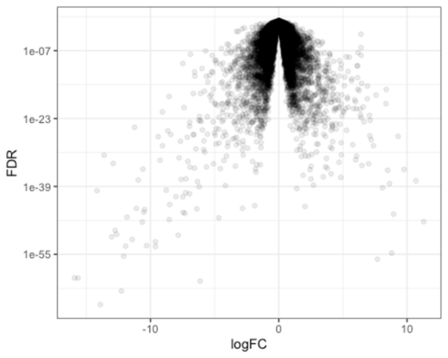
Ok, so that is most of the DE testing protocol. Note the treat function has a lfc= parameter to set the null hypothesis effect size. I left it at 0, (), meaning that some of the significant DE genes have miniscule effect sizes, and we leave it to the reader to think about which of those effects are biologically meaningful.

Power analysis through subsampling

Ok, now we have performed DE testing. The rest of this section describes how I did a power analysis (Fig1S2), wherein I subsampled reads and smaller sample sizes to understand how these subsampled smaller experiments perform in terms of power to identify DE genes and calibration of FDR. The motivation for this exercise is to better understand how to design future inter-species DE experiments to maximize power while keeping the experiment design feasible. Before I describe how I sub-sampled less reads for each library (simulating less sequencing depth), I’ll demonstrate how I subsamped smaller sample sizes.

With regards to code, it helps to wrap all of the DE analysis into a single function.

So let’s write an R function to perform the DE testing, that can take the count-table as input (pre-filtered for the outliers we want to exclude). The function will output the DE test results table. Let’s write the function so it also takes an argument (Samples) to specify which samples to include in the DE analysis. Samples will be aa character vector where entries match the column names of the CountTable. That way, we can use R’s sample function to randomly subsample samples to include when we call this function.

DE.Analysis <- function(CountTable, Samples){
  #Subsample the CountTable input by Samples
 CountTable <- CountTable[, Samples]
  
  #Define the factors and create model matrix
 SpeciesFactor <- colnames(CountTable) %>% endsWith("Human") %>% factor() %>% unclass() %>% as.character()
  mm <- model.matrix(~0 + SpeciesFactor)
  
  #estimate mean variance relationship and compute observation level weights
  y <- voom(CountTable, mm, normalize.method="cyclicloess", plot=F)
  
  #Reassign the voom expression matrix to convert from logCPM to logRPKM
  #Note that the GeneLengths dataframe is defined outside the scope of this function definition... It was defined in a previous code block.
 GeneLengths.mat <- matrix(data=NA, nrow(y$E), ncol(y$E))
  for (i in 1:ncol(y$E)){
    Species <- gsub(".+\\.(.+?)$", "\\1",colnames(y$E)[i])
    if (Species == "Human"){
     GeneLengths.mat[,i] <- GeneLengths$Length.Human
    } else if (Species == "Chimp"){
     GeneLengths.mat[,i] <- GeneLengths$Length.Chimp
    }
  }
  y$E <- y$E - log2(GeneLengths.mat/1000)
  
  #fit linear model
  fit<- lmFit(y, mm)

  #define contrasts
  contr <- makeContrasts(DE=SpeciesFactor1-SpeciesFactor2, levels = mm)
  
  #fit contrasts
  tmp <- contrasts.fit(fit, contrasts=contr)
  
  #compute test statistics, pvals
  efit <- treat(tmp, lfc = 0)
  
  #topTable function presents all the results as a nice dataframe, included FDR adjusted P.vals
  Results <- topTable(efit, n=Inf, sort.by="none")
  
  return(Results)
}

Ok, now let’s test this function…

Let’s use the CombinedTable as the CountTable input, with all 39Chimp + 39Human samples as Samples. This is in effect the same as the DE analysis we did previously with no sub-sampling. These results will be like the ‘ad-hoc gold standard’ DE results we mention in the paper, from which we can compare sub-sampled results to.

#Redefine AllSamples.CountTable, which importantly, should match
AllSamples.CountTable <- d$counts

#Preview this object
AllSamples.CountTable[1:10,1:10]

##                 4x0519.Chimp 4x373.Chimp 476.Chimp 4x0025.Chimp 438.Chimp
## ENSG00000186891           46          73        20           28         4
## ENSG00000186827          274         393       313          397       173
## ENSG00000078808         5967        1931      7637         3892      2957
## ENSG00000176022         1097         402      1574         1333       955
## ENSG00000184163            7          49       113           62        62
## ENSG00000160087          761         283      1153          776       471
## ENSG00000162572            7           4        17            2         5
## ENSG00000131584         2587        1537      3646         2546      1755
## ENSG00000169972          282          78       396          257       209
## ENSG00000127054         3009        2009      7404         3300      3600
##                462.Chimp 4X0354.Chimp 503.Chimp 317.Chimp 623.Chimp
## ENSG00000186891        11           98        13        11         3
## ENSG00000186827       128         975       236      307        84
## ENSG00000078808      3745         1189      5857     4306      3704
## ENSG00000176022      1235          416      1087      745       640
## ENSG00000184163        29          111        82        24        18
## ENSG00000160087       610          275       920      547       604
## ENSG00000162572        16           12        11         9        10
## ENSG00000131584      1323         4585      2250     1484      1872
## ENSG00000169972       282          111       243      141       252
## ENSG00000127054      2092         3147      4403     2740      3116

#Use our new function
GoldStandardResults <- DE.Analysis(CountTable = AllSamples.CountTable, Samples=colnames(AllSamples.CountTable))

#head the output to preview
head(GoldStandardResults)

##                      logFC    AveExpr         t     P.Value    adj.P.Val
## ENSG00000186891  2.6535245 -1.9348400  7.285495 1.963694e-10 1.178389e-09
## ENSG00000186827  0.6976051 1.9416561  2.841183 5.694704e-03 1.002858e-02
## ENSG00000078808 -0.2951077  5.0800668 -3.791376 2.886978e-04 6.392325e-04
## ENSG00000176022  0.1414379 2.9898884  1.837566 6.982577e-02 9.795914e-02
## ENSG00000184163  0.5987496 -0.2882371  2.532266 1.328229e-02 2.177540e-02
## ENSG00000160087 -0.1680219  2.5416948 -2.438053 1.697483e-02 2.721896e-02

Ok, let’s use our function again, but this time subsampling 10 chimps and 10 humans.

#Set seed for reproducibility when using sample function
set.seed(0)

#Subsample 10 Chimp samples
ChimpSubsample <- colnames(AllSamples.CountTable) %>%
  grep("Chimp", ., value=T) %>% 
  sample(10)

print(ChimpSubsample)

##  [1] "4X0267.Chimp"   "4x0025.Chimp"   "4x0519.Chimp"   "95A014.Chimp"  
##  [5] "4x0043.Chimp"  "570.Chimp"     "338.Chimp"     "Little_R.Chimp"
##  [9] "4X0550.Chimp"  "295.Chimp"

#Subsample 10 human samples
HumanSubsample <- colnames(AllSamples.CountTable) %>%
  grep("Human", ., value=T) %>% 
  sample(10)

print(HumanSubsample)

##  [1] "GTEX-R55G-0526-SM-2TC5O.Human" "GTEX-QLQ7-0526-SM-2I5G3.Human"
##  [3] "GTEX-OXRL-0326-SM-2I3F2.Human" "59263.Human"                  
##  [5] "63060.Human"                  "62765.Human"                 
##  [7] "62850.Human"                  "GTEX-N7MT-1326-SM-2I3FV.Human"
##  [9] "GTEX-QV44-0526-SM-2S1RE.Human" "GTEX-POMQ-0326-SM-2I5FO.Human"

#Resuse the function we made
SubSampleResults <- DE.Analysis(CountTable = AllSamples.CountTable, Samples=c(ChimpSubsample, HumanSubsample))

#Preview the SubSampledResults
head(SubSampleResults)

##                        logFC    AveExpr           t      P.Value  adj.P.Val
## ENSG00000186891  3.209334877 -2.0367354  4.06014572 0.0005285633 0.003870072
## ENSG00000186827  0.834510892 1.6431387  2.36585056 0.0273053220 0.078566328
## ENSG00000078808 -0.184752819  5.0853512 -1.08689097 0.2889543068 0.443441895
## ENSG00000176022  0.184954852 2.9547180  0.96935226 0.3429996757 0.500769220
## ENSG00000184163 -0.007835293 -0.4283833 -0.01670477 0.9868240493 0.991608386
## ENSG00000160087 -0.077855563  2.5276115 -0.58505327 0.5645177371 0.698535501

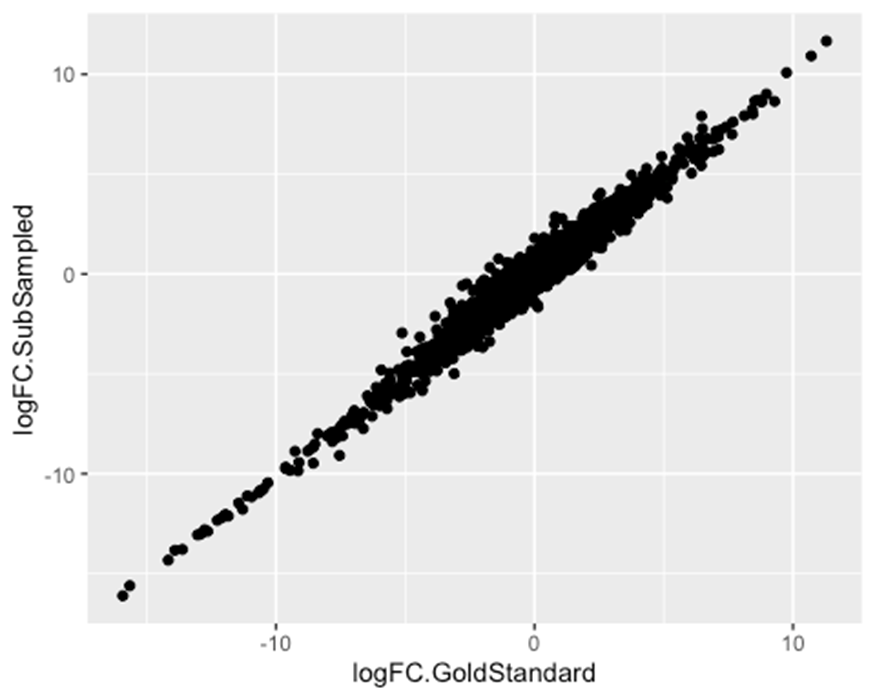
Ok, now let’s inspect how the Sub-sampled results compared to the ‘gold-standard’. There are many ways we could inspect this Fig1S2. Let’s first verify that effect sizes correlate, as a sanity check…

#Merge the two results dataframes
MergedResults <- merge(GoldStandardResults, SubSampleResults, by=0, suffixes = c(".GoldStandard", ".SubSampled"))
head(MergedResults)

##         Row.names logFC.GoldStandard AveExpr.GoldStandard t.GoldStandard
## 1 ENSG00000000003          0.9109333             1.670404      11.206591
## 2 ENSG00000000005          2.8839788            -2.205560       7.474014
## 3 ENSG00000000419          0.2782415             5.170537       3.230798
## 4 ENSG00000000457          0.3837064             1.009186       5.995548
## 5 ENSG00000000971         -1.3179363             1.996271      -6.149341
## 6 ENSG00000001036         -0.3294598             4.365151      -3.195056
##  P.Value.GoldStandard adj.P.Val.GoldStandard logFC.SubSampled
## 1        4.316553e-18          7.967760e-17        0.7547735
## 2        8.449576e-11          5.351398e-10        2.8208401
## 3        1.790438e-03          3.450506e-03        0.1367871
## 4        5.513938e-08          2.225864e-07        0.3471204
## 5        2.860967e-08          1.210218e-07       -0.7768651
## 6        1.998846e-03          3.823977e-03       -0.3272034
##  AveExpr.SubSampled t.SubSampled P.Value.SubSampled adj.P.Val.SubSampled
## 1          1.735102    4.6388322       0.0001293833          0.001284554
## 2         -1.531400    4.5351333       0.0001664504          0.001572494
## 3          5.208603    0.8006332       0.4319815346          0.586963324
## 4          1.073816    3.0284349       0.0062142956          0.025829293
## 5          2.190743   -2.1645159       0.0416500006          0.107413575
## 6          4.489680   -1.5295784       0.1404999286          0.264584860

#Plot effect size estimates between results
ggplot(MergedResults, aes(x=logFC.GoldStandard, y=logFC.SubSampled)) +
  geom_point()

Now let’s go over some of the many ways we can compare the results between the GoldStandard DE results and the Sub-sampled results.

Compare number of DE genes

#Pick some FDR threshold to call things as DE
FDR <- 0.05

#Plot number of DE genes in gold standard
sum(MergedResults$adj.P.Val.GoldStandard < FDR)

## [1] 8989

#Plot number of DE genes in Subsampled results
sum(MergedResults$adj.P.Val.SubSampled < FDR)

## [1] 4042

As expected, when we sub-sampled less samples, we got less DE genes. These numbers match Fig1S2A. As in Fig1S2A, we could have repeated this at other FDR cutoffs. But for sake of code simplicity, throughout the rest of this document we will just evaluate things at FDR=0.05.

Also note that this Sub-sampling results was just one random sampling that we could have done at this sample size. If we took another random sample of the same size, we would get slightly different results. In Fig1S2, we communicate the results of varying sample-sizes with box-whisker plots to illustrate the distribution of results from 100 random samples at each sample size. This is too computationally intensive for me to demonstrate here, but code to do so on UChicago’s parrallelized computing cluster is in the snakemake in this repo. So for the remainder of this document, I will demonstrate some code snippets to communicate the detailed methodology for the sub-panels in Fig1S2, but I will not fully recreate that figure which would require much computation than is comfortable on a laptop.

…Moving on to some of the other ways to compare the GoldStandard results to the SubSampled results, as in FigS12:

Evaluate an empirical FDR estimate

Let’s check what fraction of genes called as significant in the SubSampled set, were not significant in the GoldStandard set of DE genes (False discoveries). Let’s also account for the extreme cases where something is DE in both sets but in opposite direction (I would call that a false discovery).

#Number of total DE genes in SubSampled set
MergedResults %>%
  filter(adj.P.Val.SubSampled < FDR) %>%
  nrow()

## [1] 4042

#Number of DE genes in SubSampled set that are also DE in GoldStandard set with matching sign of effect size
MergedResults %>%
  filter(adj.P.Val.SubSampled < FDR) %>%
  filter(
     (adj.P.Val.GoldStandard < FDR) &&
      (sign(logFC.GoldStandard)==sign(logFC.SubSampled))
    ) %>%
  nrow()

## [1] 4042

In this particular random sampling subset, it seems that all 4042 DE genes identified in the subset were also DE in the GoldStandard set. This would correspond to a 0% empirical FDR. But this is just one random sampling. In Fig1S2B, for each sample size and read depth, we show the box-and-whisker distribution for 100 random samplings.

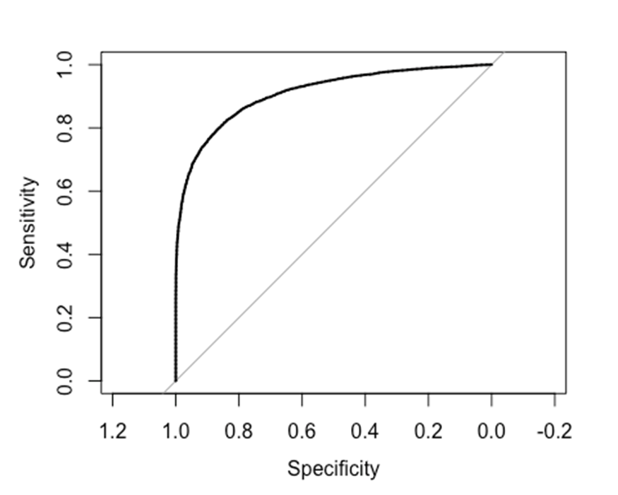
reciever operator characteristic (ROC) plot

ROC plots show the sensitivity and specificity of a binary classifier as some threshold changes. In our case, we can classify genes as DE or not DE, based on a significance threshold (p-value). So let’s create a ROC plot of the SubSampled to illustrate how well it can classify genes into their “true” responses (based on the gold-standard set of DE genes).

#Use roc function from pROC library
roc( MergedResults$adj.P.Val.GoldStandard<0.01 , MergedResults$P.Value.SubSampled, plot=T)

## 
## Call:
## roc.default(response = MergedResults$adj.P.Val.GoldStandard <    0.01, predictor = MergedResults$P.Value.SubSampled, plot = T)
## 
## Data: MergedResults$P.Value.SubSampled in 5881 controls (MergedResults$adj.P.Val.GoldStandard < 0.01 FALSE) > 7723 cases (MergedResults$adj.P.Val.GoldStandard < 0.01 TRUE).
## Area under the curve: 0.91

Ok, that looks good. But again, this is the results for just one sample, in the paper we present the results from 100 random samples at each sample size and for each point on the x-axis, we show the 5th and 95th percentile ROC curves of the random samples as a dotted line.

Effect size distribution

In Fig1S2D we show the distribution of effect sizes of DE genes. The motivating hypothesis is that for smaller sample sized experiments (eg, 4 humans vs 4 chimps), we would only be able to detect larger changes in expression. As the sample size gets bigger and bigger, we will be able to detect smaller changes in expression, so the effect sizes of DE genes should be smaller…

Note that we should be looking at the effect size as measured in the gold-standard set, not as estimated in the sub-sampled set because in smaller sub-samples, we expect that effect sizes of DE genes may be over-estimated due to winners curse effects… That is, genes which happened to have larger effect sizes in the sub-sample will be more likely to be DE genes in the sub-sample.

#Plot absolute log2FC for significant genes in each set.
MergedResults %>%
  dplyr::select(Row.names, adj.P.Val.GoldStandard, adj.P.Val.SubSampled, logFC.GoldStandard) %>%
  gather(key = "DE.Analysis", value="adj.P", adj.P.Val.GoldStandard, adj.P.Val.SubSampled) %>%
  filter(adj.P < 0.05) %>%
  ggplot(aes(x=DE.Analysis, y=abs(logFC.GoldStandard))) +
  geom_boxplot(outlier.shape = NA) +
  scale_y_continuous(limits=c(0,5)) +
  theme_bw()

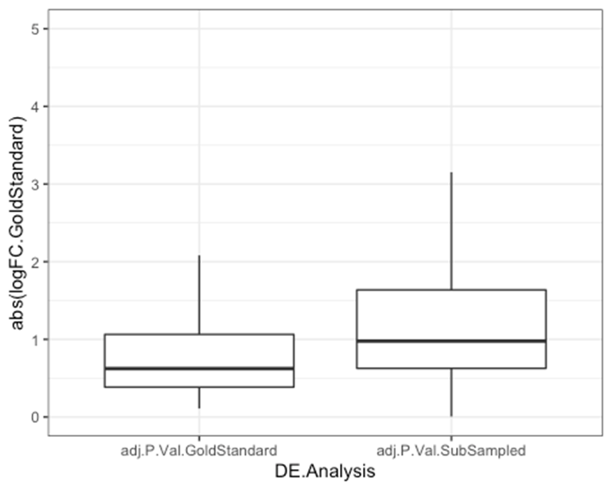
As expected, and as shown more extensively in Fig1S2D, when we use a smaller sample size, we detect DE genes for genes with larger true changes. In Fig1S2D, rather than show the results for 100 random samples at each sample size (which I could not come up with a intuitive way to plot), I just picked the median iteration at each sample size in terms of number of DE genes, and plotted the distribution of effect sizes for that iteration.

Quantifying winner’s curse effects

As described above, especially at smaller sample sizes, effect sizes tend to over-estimated when selecting from discoveries that pass some signifcance threshold. See Ionnidis 2008. This is statistical theory. Fundamentally, the problem comes from double dipping the data to perform inference and estimation from the same dataset. Once we perform inference to select genes, if we want to estimate effect sizes without bias, we should technically use an independent data set. Obviously in genomics (and especially in comparative primate genomics), sometimes obtaining independent data is not feasible. In FigS2E we wanted to quantify how strong this bias was as a function of sample size. Here is some code to demonstrate, using our single random sample at sample-size=10 compared to the gold-standard set.

#Get the median difference in log2FC for DE genes
MergedResults %>%
  filter(adj.P.Val.SubSampled < FDR) %>%
  mutate(DifferenceInEffectSizeEstimate = logFC.GoldStandard - logFC.SubSampled) %>%
  pull(DifferenceInEffectSizeEstimate) %>%
  abs() %>%
  median()

## [1] 0.1319121

So that is to say, that when using sampleSize=10, we can expect that a typical effect size estimate (log2FC) for a DE gene (at this FDR<0.05 theshold), is over-estimated by 0.13!

In FigS2E, we show the box-and-whisker distribution of results for 100 random draws at each sample size.

Evaluating contribution of read depth.

So far, we have been using all of our samples with the full read depth that we sequenced in our experiment, which varies from >25M to >80M reads mapped to genes. But would our results change substantially if we controlled sequencing depth to exactly 25M reads per sample. Or perhaps less? What about 10M reads per sample. In Fig1S2 I repeat the results for A-E after sub-sampling less reads for each library to simulate less sequencing depth. In short, the conclusion is that the sequencing depth doesn’t play nearly as large a role as sample size. In theory, one could write a function to sub-sample counts from the count-table, but I couldn’t think of a good way to code that. In the end, I found it just simpler to sample reads from the original bam files for each sample:

samtools view -bh -s {FractionOfReadsOfReadsToSubsampleFromInputBam} {inputBam} > {SubSampledOutputBam}

and then re-made count-tables using featureCounts from sub-sampled bam files. In Fig1S2, I sub-sampled bams such that library file would have either 25M or 10M reads. Because some libraries have different gene-mapping rates, I first had to determine the gene-mapping rate for each file such that when I sub-sample a fraction of reads with -s {FractionOfReadsOfReadsToSubsampleFromInputBam} I would end up with a fixed number of gene-mapped reads each sample. The code for doing so is also in the snakemake in the git repo, and the results of sub-sampled featureCounts output are tracked in the git repo as:

https://github.com/bfairkun/Comparative_eQTL/blob/master/output/PowerAnalysisCountTable.Chimp.10000000.subread.txt.gz

and similarly named files.

Conclusions

Hopefully this was useful in some way to somebody =).

Again, a lot of these results (particurly the power analysis in Fig1S2) may not exprapolate well to different tissues or different species. But still in general, I feel like I learned a bit doing this analysis: In particular I learned that:

• More samples is more power (duh)
• Even only 10M reads per sample is fine, what really gives more power is more samples moreso than more reads per sample
• FDR seems to be actually decently calibrated… Of course, we were defining the “true” response by the significant genes when samples size is 38H+38C, and at some level (with large enough sample size), every gene is DE… So what does FDR even mean? This could devolve into more into FalseDiscoveryRate versus FalseSignRate, or more generally to null hypothesis testing paradigm, versus putting more emphasis on effect size estimation… Anyways..
• Winner’s curse bias is real. Be aware that effect size estimates of DE genes are inflated, especially at smaller sample sizes (Fig1S2E)

Category