


- Protocols

- Articles and Issues
- For Authors
- About
- Become a Reviewer


Automated FLIM-FRET Segmentation Within RNP Condensates

(*contributed equally to this work) Published: Vol 16, Iss 15, Aug 5, 2026 DOI: 10.21769/BioProtoc.5775 Views: 377
Reviewed by: Maya V RaoAleksandra J. WierzbaAnonymous reviewer(s)
 PDF
PDF  Ask a question
Original research article
The authors used this protocol in:

Oct 2024

Protocol Collections
Comprehensive collections of detailed, peer-reviewed protocols focusing on specific topics




Abstract
Ribonucleoprotein (RNP) condensates are membraneless organelles that exist alongside many RNA-driven processes, such as transcription and splicing. Despite their ubiquity, the biological necessity of forming a condensed phase remains unclear, particularly because the same RNP components exist both within these organelles and in the surrounding dilute phase. Most current methods for studying biochemical interaction dynamics within condensates rely on in vitro reconstitution of minimal factors or low-throughput single-molecule studies. However, RNP condensates are complex organelles containing tens to hundreds of proteins and hundreds to thousands of different RNAs. Here, we describe a scalable, high-throughput fluorescence microscopy–based approach to analyze protein–protein interaction networks, allowing for the rigorous assessment of dynamic, process-critical interactions within RNP condensates from live cells. This method takes advantage of fluorescence lifetime imaging (FLIM) and phasor plot analysis to automate segmentation of condensate-localized fluorescence signals. Using suitable FLIM–Förster resonant energy transfer (FLIM-FRET) fluorescent pairs fused to proteins of interest, protein–protein interactions can be actively monitored throughout various conditions via changes in fluorescence lifetime. Results from this assay yield valuable insight into the organization and assembly of essential factors for different condensate-associated processes to infer the functional consequences of RNP granule partitioning. Although this protocol is tailored for studying protein interactions within condensates, the design and execution framework can be adapted to investigate protein–protein interactions across a wide variety of compartments within different biological systems.
Key features
• Automated segmentation of condensate-localized fluorescent signal independent of thresholding or background subtraction.
• FLIM-FRET to analyze protein–protein interactions, with an emphasis on condensate interaction networks.
• Monitor protein interactions from live cells over time and in response to different stimuli.
Keywords: Fluorescence lifetime imaging microscopy Förster resonance energy transfer
Segmentation
Condensates
Phasor analysis
Förster resonance energy transfer
Segmentation
Condensates
Phasor analysis
Graphical overview
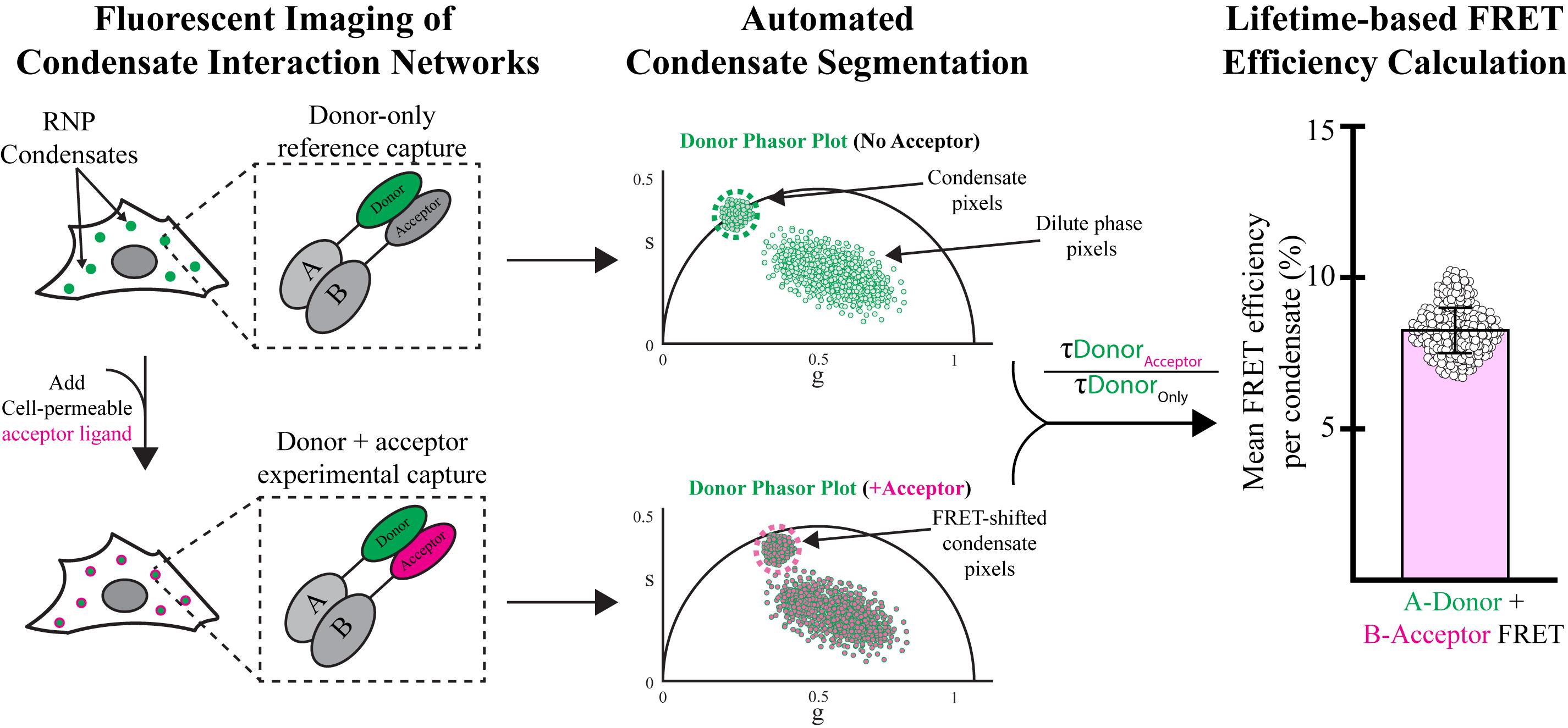
Graphical overview of fluorescence lifetime imaging–Förster resonant energy transfer (FLIM-FRET) capture, segmentation, and analysis
Background
Uncovering protein–protein interaction networks can yield valuable mechanistic insight into the function of various biological systems. However, many biochemical approaches, such as co-immunoprecipitation, lose critical spatial information that is necessary for interpreting function. This is important since many proteins specifically localize to multiple places to perform distinct functions (Figures 1C and 2). For instance, certain cytosolic proteins can be recruited to membrane-bound organelles in a context-dependent manner, such as Lsg1 interacting with VAPB at the endoplasmic reticulum membrane during oxidative stress (Figure 2A). Additionally, proteins found in ribonucleoprotein (RNP) condensates display dual localization that is technically challenging to disentangle.
RNP condensates are membraneless organelles that arise through phase separation and are classified by the specific RNA and protein species they contain [1,2]. Constituent components of these organelles are partitioned into condensed (inside the condensate) and dilute (outside the condensate) phases that rapidly exchange with one another. This unique biophysical phenomenon can allow for emergent biology [3]; however, the exact function of many condensates remains unclear. Due to the dynamic component exchange, identifying fluorescence microscopy foci as phase-separated compartments and disentangling processes that occur within the condensed phase vs. the dilute phase remain challenging. Current approaches include descriptive microscopy (size, number, shape, etc.), isolation of granules followed by sequencing [4–6], condensate reconstitution using purified components [7,8], or proximity-labeling approaches [9]. Although informative, these approaches either fundamentally alter the physical/compositional properties of the organelle or only provide descriptive information rather than mechanistic insight. To overcome these challenges, we developed a fluorescence lifetime imaging (FLIM)-based assay that allows for the automated segmentation of condensate-specific molecules to assess their functional organization in live cells using Förster resonance energy transfer (FRET) (Figures 1 and 2). Furthermore, this approach is broadly applicable to any number of biological systems to spatiotemporally interrogate protein–protein interaction networks, independent of localization (Figure 2A).
FRET is a light microscopy technique that measures protein–protein interaction networks based on energy transfer between two fluorescently tagged proteins of interest—one fused to a donor fluorophore and the other to an acceptor fluorophore. In this system, the emission spectrum of a donor fluorophore overlaps with the excitation spectrum of an acceptor fluorophore. When the two molecules interact, their fused fluorophores become close enough in proximity that energy from the excitation of the donor can transfer to the acceptor [10]. The efficiency of energy transfer is then a function of the brightness of the donor fluorophore, the degree of spectral overlap between the donor and acceptor, and the distance between donor and acceptor [10].
In classical FRET, this interaction can be quantified by measuring the loss of donor signal in the presence of an acceptor, by detecting acceptor emission directly, or by observing an increase in donor fluorescence upon photobleaching the acceptor. However, many factors can confound intensity-based measurements, including photobleaching and spectral bleed-through. Multiple methods of quantification are often necessary to confidently identify FRET, including acceptor photobleaching, which is destructive and prevents repeated measurements from the same sample over time [11]. As a result, intensity-based FRET is limited by the need for instrumentation capable of spectrally separating donor and acceptor signals, the use of photostable and high quantum yield fluorophores, and sufficiently high concentrations of both labeled species for FRET efficiency calculations [11].
To overcome many of these challenges, fluorescence lifetime imaging microscopy (FLIM) can be implemented in combination with FRET (FLIM-FRET). FLIM is a technique that measures both the fluorescence intensity and lifetime of a particular fluorescent molecule. Upon protein–protein interaction, energy transfer to the acceptor fluorophore decreases the donor fluorescence lifetime [12]. This means FLIM-FRET only needs to measure the donor lifetime and is independent of fluorophore concentration. Furthermore, FLIM-FRET avoids the need to photobleach the acceptor fluorophore and negates acceptor cross-excitation. Conjugated fluorescent tags, such as those used with Halo-tag or SNAP-tag ligands, are particularly well-suited as FRET acceptors in this system, since they allow a single cell line to serve as both a donor-only control and a donor-plus-acceptor experimental condition. Lastly, because this approach is non-destructive, multiple measurements can be acquired from the same sample over time, enabling detection of dynamic changes in protein–protein interaction.
Not only does FLIM improve FRET measurements, but we have also leveraged this imaging technique to automatically segment condensate-specific FRET signals. Standard intensity-based condensate segmentation relies on manual curation of various thresholding algorithms to distinguish condensed pixels from non-condensed pixels. These approaches assume that the bright foci of a fluorescently tagged condensate protein are the only bona fide condensates present. This results in under-counting the true number of granules or falsely identifying other structures (like lysosomes) as condensates. Fluorescence lifetime is sensitive to aspects of the microenvironment, such as pH [13], ion density [14], and, as we recently discovered, residency within condensates [15]. The reason for this condensate-specific lifetime shift is currently unclear but has been reported by others [16,17]. We hypothesize that the dense condensate environment might alter lifetimes by suppressing the non-radiative decay of certain fluorophores. This may occur through viscosity-dependent inhibition of chromophore isomerization and/or local water depletion within the condensate [18–21]. Regardless, by exploiting the subtle changes in lifetime, we developed a segmentation method to isolate fluorescence lifetime signals specifically within condensates.
Automating the segmentation of microscopy images using fluorescence intensity has been historically challenging, especially with factors that reside in multiple locations within the cell. This is particularly a problem for condensates whose dilute phase signals complicate automated thresholding of condensate pixels from dilute phase pixels during standard intensity-based segmentation. FLIM imaging provides a complementary approach that can organize pixels by fluorescence lifetime on phasor plots. FLIM phasor plots are generated by applying a Fourier transformation to the fluorescence decay curves of each pixel from time-correlated single-photon counting data (TCSPC) [22] (Figure 1D). Each pixel from the original image is represented as a single point on the phasor plot such that pixels with similar lifetime compositions cluster together (Figure 1D). Pixels with a single, uniform local environment yield mono-exponential decay signatures that cluster on the universal circle, whereas pixels with two or more distinct lifetime species (mixed microenvironments, multiple fluorophores, autofluorescence, or shot noise) yield multi-exponential decay curves and cluster inside the universal circle. Importantly, fluorescence lifetime clusters on FLIM phasor plots are amenable to a variety of automated segmentation and signal processing approaches [23,24].
To segment RNP condensates, we used FLIM phasor plots to exploit lifetime and intensity differences between condensed and dilute phases. Condensate localized pixels cluster on the universal circle because they are dominated by the fluorophore’s mono-exponential decay. Dilute phase pixels contain a mixture of lifetimes representing fluorophore, autofluorescence, and shot noise, which is proportional to the square root of the photon counts, resulting in multi-exponential decay. To resolve overlapping condensed and dilute phase lifetime clusters, we implemented a complex wavelet filter [15,24]. Following wavelet filtering, the enriched condensate lifetime cluster can be statistically isolated using a Gaussian mixture model (GMM) with a region of interest (ROI) defined by the probability distribution density of the GMM-identified lifetime cluster. A reverse Fourier transform is then applied pixel-to-pixel to map the segmented phasor coordinates back into the spatial domain, yielding accurate masks of RNP condensates.
This phasor-based segmentation can then be combined with FLIM-FRET to gain previously unattainable insight into condensate organization and function. For demonstration, we show how FLIM-FRET can be used to measure the interaction between the P-body-localized mRNA decapping proteins Dcp2 and Dcp1A/Dcp1B. Furthermore, we show how mNeonGreen and Halo-Tag conjugates can be used in this system to measure condensate protein–protein interactions within a single cell line. However, this FLIM-FRET method can also be applied to a variety of other protein factors (regardless of localization) using any FRET-capable pair of fluorescent molecules.
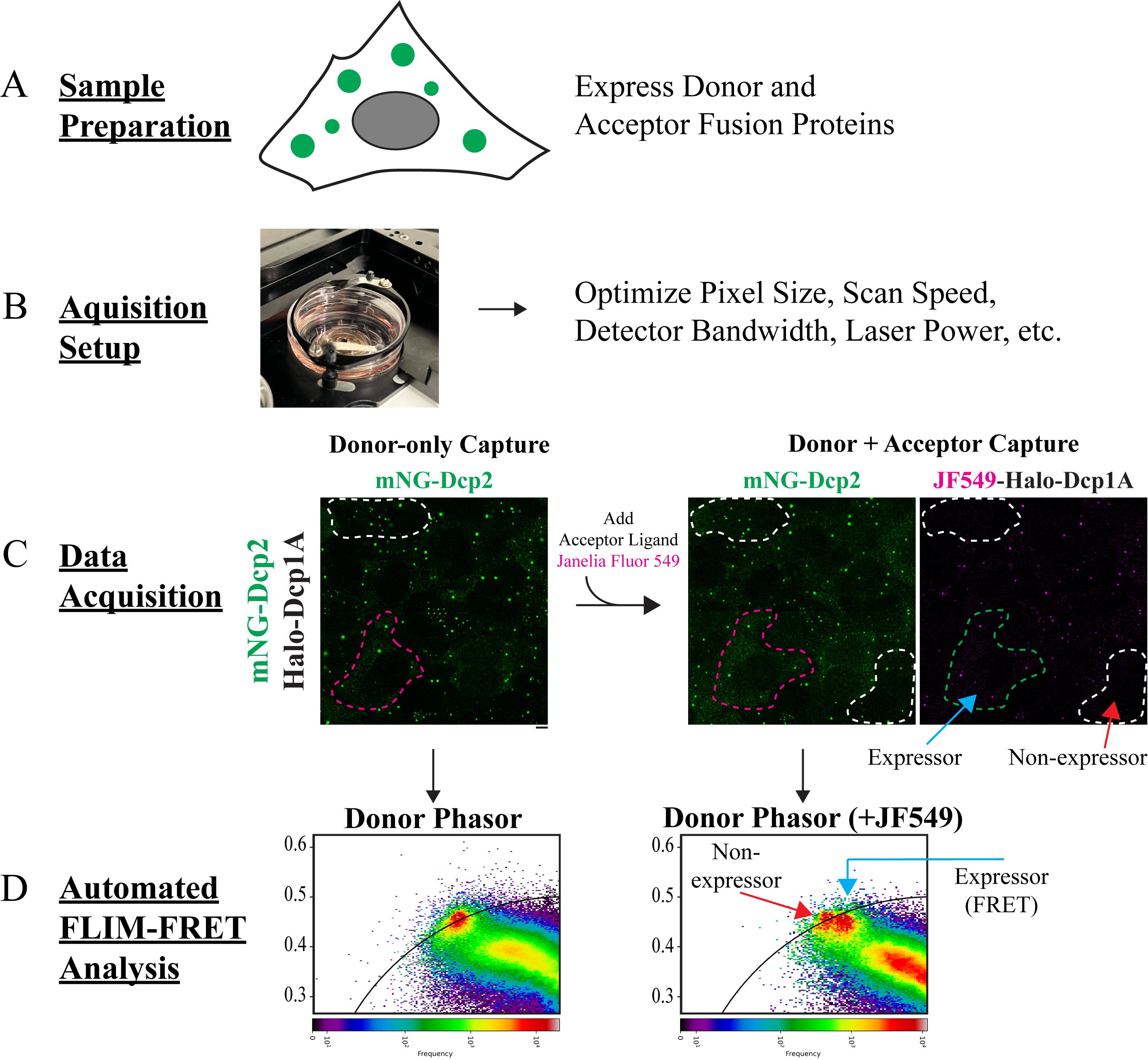
Figure 1. Overview schematic of fluorescence lifetime imaging–Forster resonant energy transfer (FLIM-FRET) data acquisition procedure. (A) Prepare samples with the cell line of interest expressing the protein–protein interaction pair of interest. One FRET partner is fused to a donor fluorophore, and the other is fused to a fluorescently conjugatable protein tag (such as HaloTag or SNAPtag) as the acceptor. (B) Set up image capture settings and optimize fluorescence intensity by adjusting pixel size, scan speed, detector bandwidth, and laser power. (C) Capture two separate donor-only and donor + acceptor images for quantification. For demonstration purposes, U-2 OS cells expressing mNeonGreen-Dcp2 as the donor and HaloTag-Dcp1A as the acceptor are shown. For illustrative purposes, green and magenta dotted outlines indicate cells that express both donor and acceptor FRET pairs. White dotted outlines indicate cells that only express the donor. Scale bar = 10 μm. (D) The final step is to process FLIM data by generating phasor plots and measuring decreases in donor fluorescence lifetime after addition of the acceptor ligand. A positive FRET signal is indicated by a clockwise shift in cluster position on the phasor plot. Microscopy images and representative phasor plots are adapted from [15].
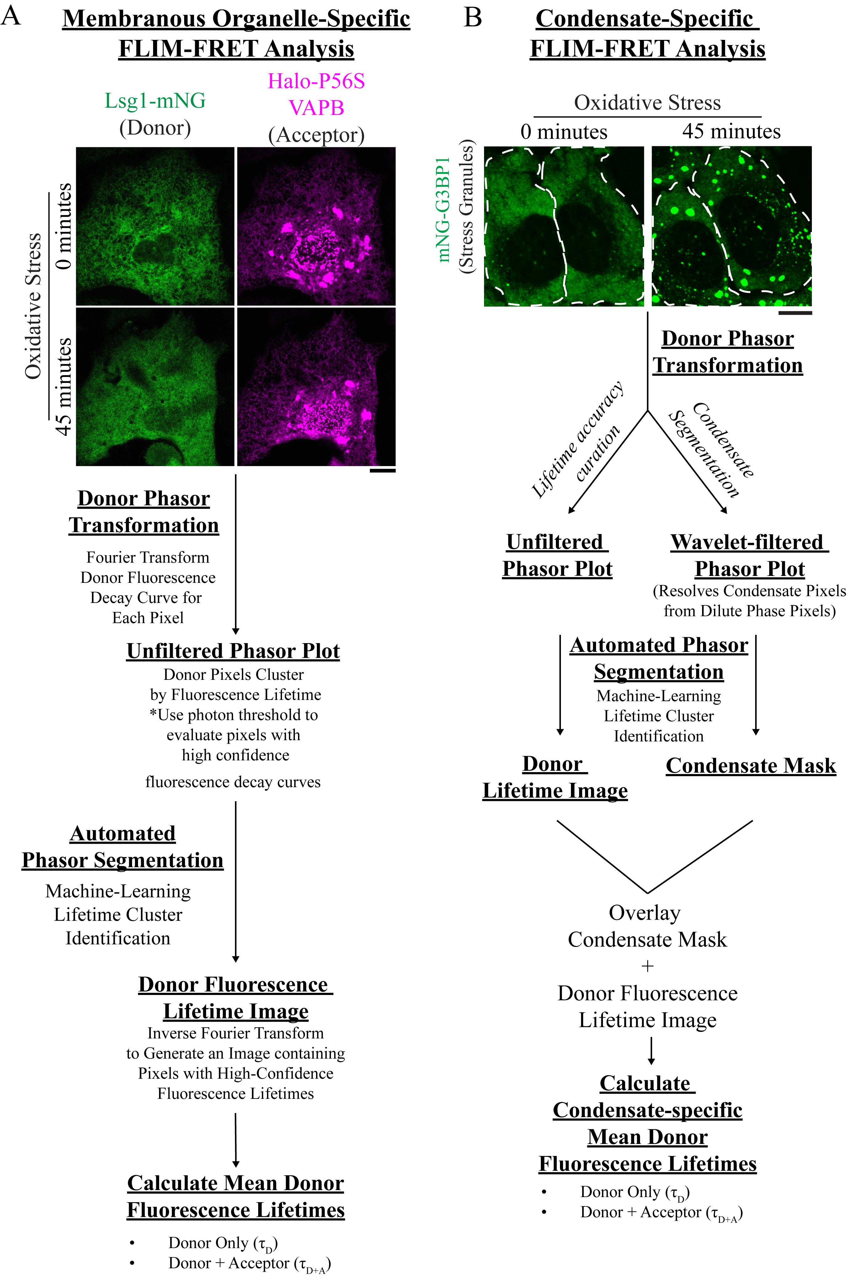
Figure 2. Overview of the fluorescence lifetime imaging (FLIM) data processing and Forster resonant energy transfer (FRET) analysis pipelines. (A) Post-acquisition FRET analysis procedure for FRET pairs that localize to membrane-bound organelles. The example illustrates two proteins, Lsg1 and VAPB, that localize to the endoplasmic reticulum during stress. However, the P56S mutant form of VAPB fails to recruit Lsg1 to the endoplasmic reticulum after 45 min of oxidative stress (500 μM NaAsO2). Scale bar = 10 μm. This analysis pipeline is a simplified version that does not require wavelet-based segmentation. (B) Post-acquisition FRET analysis procedure for FRET pairs that localize to condensates (membraneless organelles). The presented example shows how G3BP1, a core stress granule component, localizes into stress granules in response to oxidative stress (500 μM NaAsO2). This necessitates an additional phasor-based condensate segmentation step in combination with the lifetime measurements shown in A. Microscopy images of stress granules are adapted from [15].
Materials and reagents
Biological materials
1. Cell line of interest expressing donor-tagged and acceptor-tagged interaction pairs
Note: Here, for demonstration purposes, we use U-2 OS cells (ATCC, catalog number: HTB-96) stably expressing mNeonGreen-Dcp2 and HaloTag-Dcp1A or HaloTag-Dcp1B. However, this protocol can be adapted to work with any FRET-capable pair of fluorescent proteins fused to any two proteins of interest (see General note 1).
Reagents
1. Janelia Fluor® 549 HaloTag® ligand (Promega, catalog number: HT102A)
2. McCoy’s 5a medium (Sigma-Aldrich, catalog number: M8403)
3. GlutaMAXTM supplement (Gibco, catalog number: 35050061)
4. FBS, Opti-Gold (Genedepot, catalog number: F0900-050)
5. Penicillin-streptomycin 10,000 U/mL (Gibco, catalog number: 15140122)
6. Trypsin-EDTA (0.05%), phenol red (Gibco, catalog number: 25300062)
7. Phosphate buffered saline (PBS) 20×, ultrapure (VWR, catalog number: E703)
8. N, N-Dimethylformamide (Sigma-Aldrich, catalog number: 227056)
9. Type F immersion liquid (Leica Microsystems, catalog number: 11513859)
Solutions
1. Complete McCoy’s 5a medium (see Recipes)
2. Janelia Fluor® 549 HaloTag® ligand stock (see Recipes)
Recipes
1. Complete McCoy’s 5a medium
| Reagent | Final concentration | Quantity or volume |
|---|---|---|
| McCoy’s 5a medium | 88% | 440 mL |
| Penicillin-streptomycin (100×) | 1% | 5 mL |
| GlutaMAXTM supplement (100×) | 1% | 5 mL |
| FBS, Opti-Gold | 10% | 50 mL |
2. Janelia Fluor® 549 HaloTag® ligand stock
| Reagent | Final concentration | Quantity or volume |
|---|---|---|
| Janelia Fluor® 549 HaloTag® ligand | 14 µM | 5 µg |
| N, N-Dimethylformamide | n/a | 70 µL |
Aliquot in small volumes to avoid freeze-thaw cycles. Store at -20 °C.
Laboratory supplies
1. 35 mm micro-well dishes (Cellvis, catalog number: D35-14)
2. 6 cm cell culture dishes (VWR, catalog number: 10861-658)
3. 5 mL serological pipettes (Corning, catalog number: CLS4251)
4. 10 μL pipette tips (VWR, catalog number: 613-6440)
5. Microcentrifuge tubes (VWR, catalog number: 87003-294)
Equipment
1. Confocal microscope (Leica, model: Stellaris 8 FALCON)
2. 63× objective (HC PL APO CS2 63× 1.40 N.A. Oil Immersion Objective, Leica, model: 15506350)
3. 78 MHz pulsed white light laser (WLL, 440–790 nm) (Leica, model: 158301100)
Note: A slower pulsed laser (e.g., 40 MHz) may also be used to more accurately detect fluorescent proteins with longer lifetimes. See General note 2.
4. HyD X detector (Leica, model: 158301324)
5. HyD R detector (Leica, model: 158301335)
Note: Non-hybrid detectors can also be used to collect lifetime data, so long as they can record single photon events (e.g., MCP-PMT or SPAD detectors)
6. Stage top incubation system and objective heater (Okolab, model: H301)
Note: Any stage top incubator can be used, so long as it can maintain physiological conditions to support the desired cell system (e.g., 37 °C, 5% CO2, and 90% humidity)
7. Pipette controller (VWR, model: 613-4448)
8. Class II biosafety cabinet (Labconco, catalog number: LCN 302481101)
9. CO2 incubator (PHCBI, catalog number: MCO-170AICUVDL-PA)
10. 10 μL micropipette (Eppendorf, catalog number: EP3124000016)
Software and datasets
1. Leica Application Suite X (LAS X, Leica Microsystems)
2. Leica Application Suite X FLIM (LAS X, Leica Microsystems)
3. FLUTE (open source) [25]
4. FIJI/ImageJ (open source)
5. Microsoft Excel
6. ComplexWaveletFilter [open source, system requirements: MacOS 10.9 (Mavericks) or later, Python v3.6.0], release date: December 23, 2025. This code has been deposited to GitHub (https://github.com/LeeLabBCM/ComplexWaveletFilter) and archived on Zenodo (DOI: 10.5281/zenodo.20631326; release v1.0.0).
Procedure
A. Sample preparation
1. Culture U-2 OS expressing mNeonGreen-Dcp2 and HaloTag-Dcp1A cells in complete McCoy’s 5a medium in 6 cm cell culture dishes at 37 °C, 5% CO2, and 95% humidity. Allow cells to reach 80%–90% confluency.
2. At least 24 h prior to imaging, seed cells into one 35 mm glass-bottom dish.
a. Remove media from the 6 cm culture dish.
b. Wash the cells with 3 mL of PBS to remove any residual media.
c. Detach cells by adding 1 mL of trypsin and incubate at 37 °C for approximately 3 min or until cells lift off the dish.
d. Neutralize trypsin by adding 4 mL of complete McCoy’s medium and plate approximately 100,000 cells into one 35 mm microscope dish.
3. Allow cells to attach at 37 °C, 5% CO2, and 95% humidity in the incubator overnight.
B. Microscope setup and capture settings
Note: This example experiment is performed using the Leica Stellaris 8 FALCON confocal system. Any time-domain FLIM system can be used as long as the time-correlated single-photon counting (TCSPC) data can be exported and converted to .tiff file format. FLIM-FRET only requires recording of the donor fluorescently tagged protein, but it is also important to capture representative images of the acceptor protein to confirm proper acceptor localization. The downstream analysis workflow requires single-channel FLIM capture. Therefore, to record fluorescence intensity of both donor and acceptor proteins (to confirm donor and acceptor colocalization) and record FLIM for the donor protein, it is necessary to set up two modes of data acquisition for FLIM and non-FLIM fluorescence intensity.
1. Prepare the microscope for live imaging. Turn on the microscope, stage top incubator system, white light laser, computer, and CO2. Allow the chamber to reach 37 °C, 5% CO2, and 95% humidity.
2. Start the LASX software. When prompted, tilt the transmitted light arm back to allow the stage to initialize.
3. Set the confocal imaging settings. The main LASX window has three panels: a left-side panel for confocal and capture settings, a center panel for light path settings, and a right-side panel for viewing images. Click the FLIM button under the acquisition tab on the left-side panel to launch the FLIM software (Figure 3A).
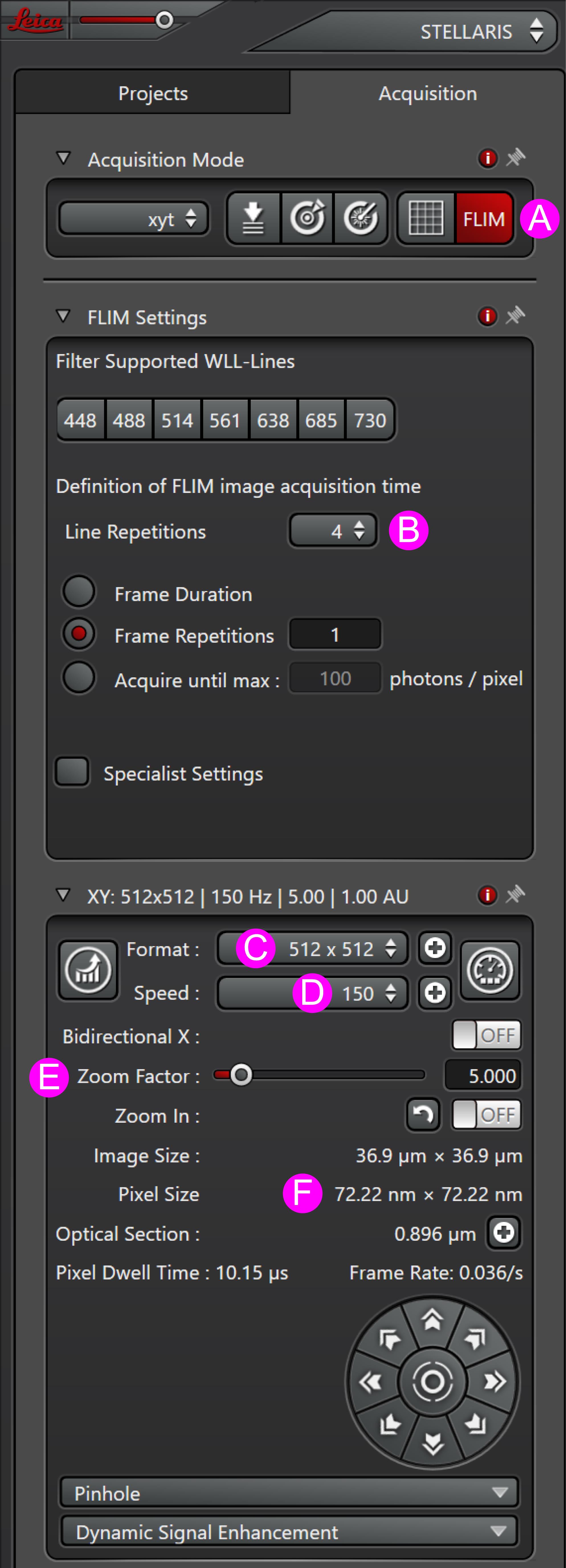
Figure 3. Capture settings panel in LAS X software. This is the location in the LAS X user interface where confocal and FLIM capture settings are set. (A) Button to turn on FLIM capture mode. (B) Drop-down menu to set line repetitions for FLIM capture. (C) Drop-down menu to set the confocal scan format. (D) Drop-down menu to set the confocal scan speed in Hz. (E) Slider to set the zoom factor. (F) Pixel size calculated from scan format, zoom factor, and objective magnification and numerical aperture.
4. Configure the following capture settings in the LASX capture settings panel for FLIM imaging:
a. 512 × 512 scan format (Figure 3C).
Note: 512 × 512 scan format is included here as this is the highest pixel format that is computationally viable for the Stellaris 8 FALCON system. Different systems may have alternative maximum pixel formats. Reducing scan format will increase pixel size, which results in a reduction in resolution but an increase in signal per pixel. This, along with the zoom factor, can be adjusted to optimize resolution and signal detection in a given system (see Troubleshooting 1).
b. Adjust the zoom factor to the optimal pixel size. We use 72.22 nm ×72.22 nm pixel size (Figure 3E–F).
Note: Zoom factor can be adjusted according to the desired resolution, so long as the scan format does not exceed the maximum range for a given FLIM system. Pixel size will vary depending on the objective and FLIM system being used (we use a 63× 1.40 N.A. objective and a zoom factor of 5.0).
c. 150 Hz scan speed (Figure 3D).
d. 4 line repetitions (Figure 3B).
Note: Line repetitions is the same as line accumulation in the LASX software.
5. Set the light path for capturing mNeonGreen for FLIM imaging from the center light-path panel of LASX (Figure 4). Make sure the line scanning mode is turned on (Figure 4B).
a. Click the Add Laser button (Figure 4C) once and then click on a setting window. A black bar will appear with a number indicating the laser line wavelength. Double-click that bar to change the laser line wavelength and power. Set the white light laser line to 504 nm and 5% laser power.
b. Double-click on the detector window icon at the bottom of the capture setting window (Figure 4E) to change detector window settings. Use the HyD X3 and set the detector window from 520 to 550 nm. Use the drop-down menu under Operation Mode to set the detector to counting mode (Figure 4F).
6. For standard confocal imaging (to attain representative colocalization images of donor and acceptor, not FLIM data), configure the capture settings (Figure 3) and light path settings (Figure 4) as follows:
a. 512 × 512 scan format.
b. 72.22 nm × 72.22nm pixel size.
c. 400 Hz scan speed.
d. 1× line accumulation.
Critical: Oversampling of the donor channel can result in inaccurate lifetime measurements. The signal needs to be high enough to obtain at least 100 photons per pixel intended to be analyzed, but must remain below 1 photon per laser pulse. This is important for accurate fluorescence lifetime calculations. In the FLIM module of LASX, a histogram plot of photons per laser pulse is propagated with a red line at 1 to indicate the upper limit for photon detection. Adjust laser power, line accumulation, scan speed, or detector windows such that the histogram remains below 1 photon per laser pulse.
7. Set two light paths to capture mNeonGreen and HaloTag labeled with Janelia Fluor 549 for confocal imaging (Figure 4):
a. Set up light path setting #1 with white light laser at 570 nm with 6% laser power, HyD R4 detector window from 585–740 nm, and set to counting mode.
b. Set up light path setting #2 with white light laser at 504 nm with 6% laser power, HyD X3 detector window from 520–550 nm, and set to counting mode.
Note: To save time switching back and forth between FLIM capture mode and confocal capture mode, save a configuration file of each light path that can be quickly loaded.
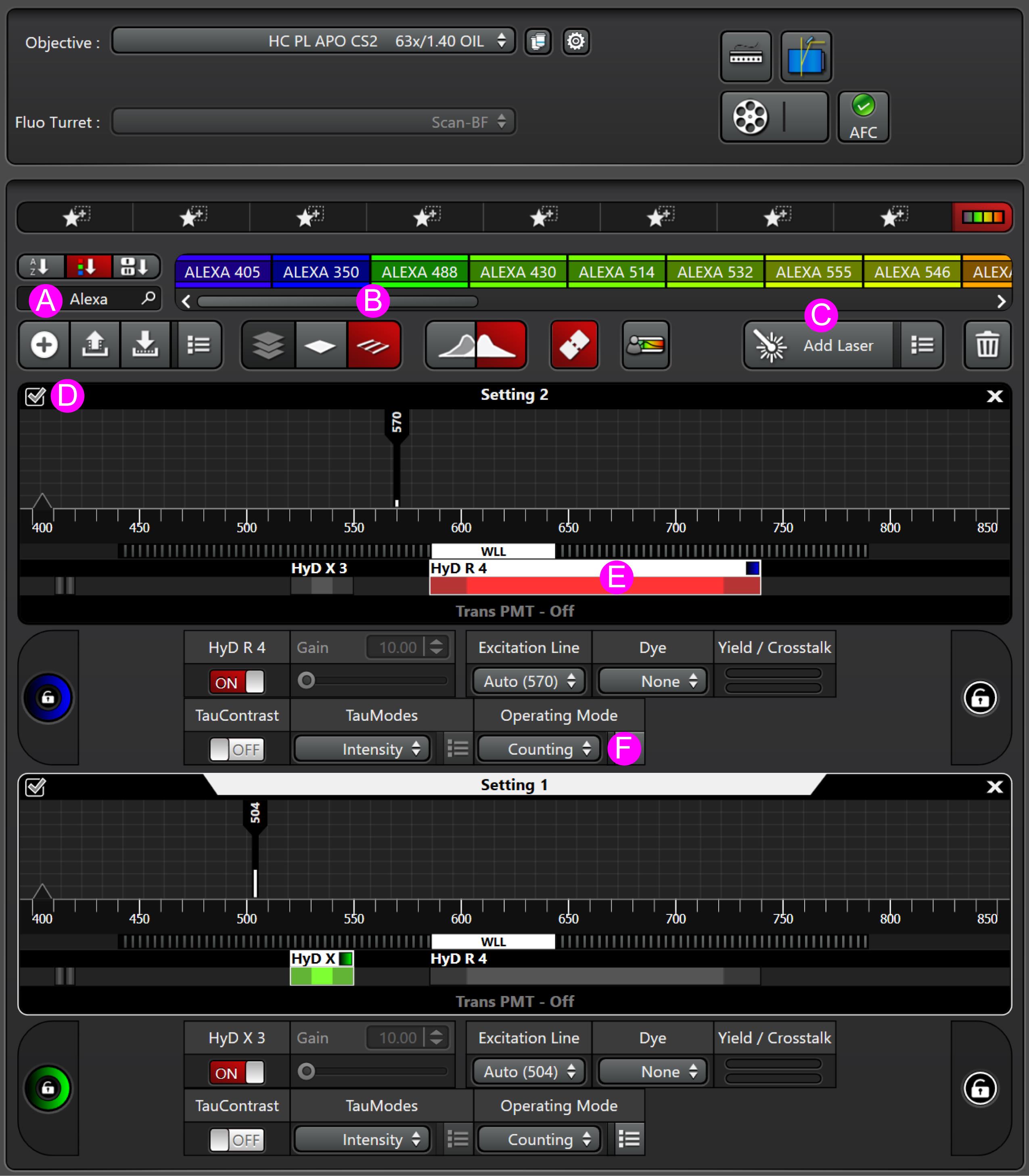
Figure 4. Light path panel in LAS X software. This is the location in the LAS X user interface where light path settings are set. (A) Button to add a light path setting. (B) Indicator that line scanning mode is turned on. (C) Button to add a white light laser line to a light path setting. (D) Check box to toggle a light path setting on or off. (E) Detector window. (F) Drop-down menu to select detector counting mode.
C. FLIM live-cell image capture
Note: Since the example experiment uses a cell-permeable conjugatable ligand (Janelia Fluor 549), proper labeling is critical for recording consistent FRET measurements. The following steps have been optimized for Janelia Fluor HaloTag ligands. Other protein handles (such as SNAPtag) and their corresponding ligands may be used, but should be optimized to ensure complete and consistent labeling. See General notes 1 and 3 for FRET systems using constitutively fluorescent molecules as the acceptor instead of conjugatable protein tags.
1. Lower the objective and add a small drop of oil directly onto the objective lens. Place one of the dishes in the stage top incubator and secure the dishes in the incubator with magnetic clamps (Figure 5).
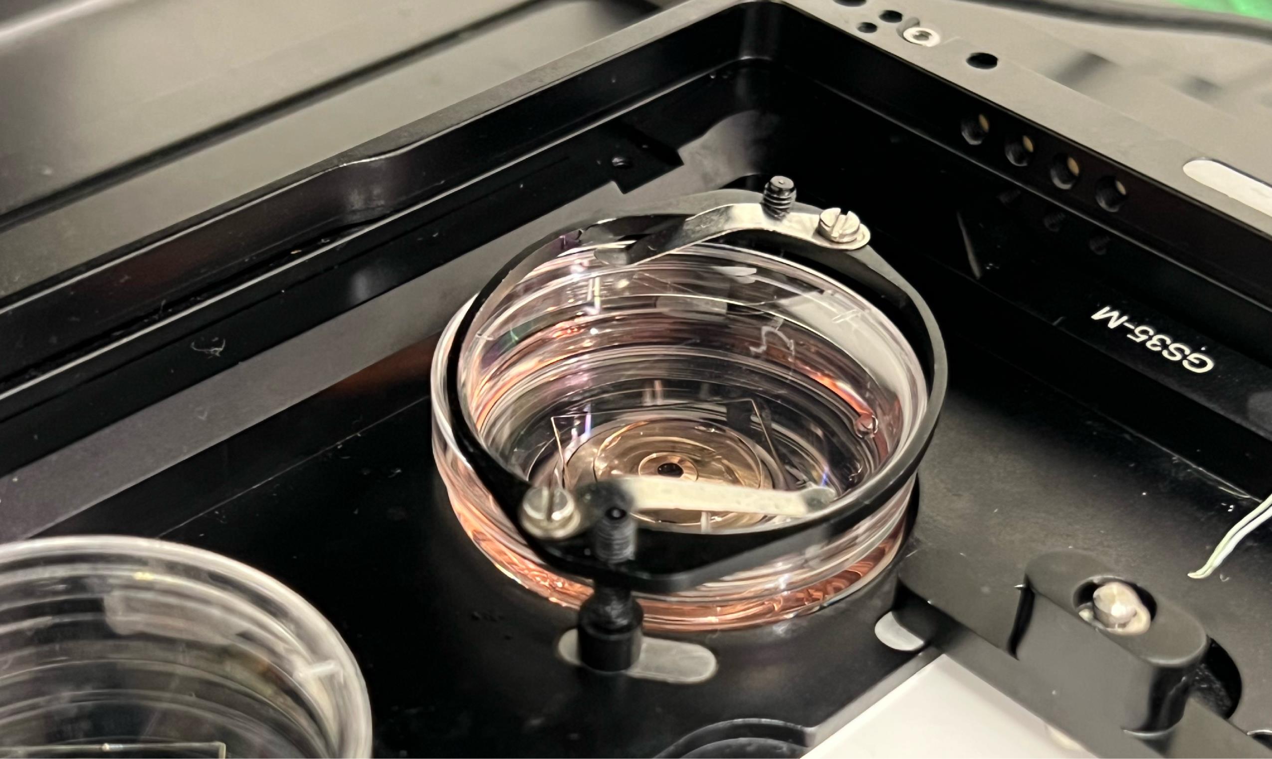
Figure 5. Stage top incubator system. Magnetic clamps used to secure a dish in the incubator unit.
2. Use the eyepiece to find a general focus before locating the precise focal plane using the Fast Live function within LASX software.
Note: Avoid the use of epifluorescence light as much as possible because photobleaching can negatively affect FLIM measurements.
3. Capture first with the FLIM capture settings from steps B4–5.
Critical: For the data analysis workflow, it is essential that FLIM is captured as a single channel.
4. Then, capture with the confocal capture settings from steps B6–7.
5. Add a final concentration of 14 nM Janelia Fluor 549 HaloTag ligand to the media.
Critical: Ideally, the same cells will be imaged for donor and donor + acceptor captures. Therefore, avoid bumping or moving the dish when adding the ligand.
Critical: Do not add the ligand directly on top of the cells, as this may result in background staining. Add to the edge of the dish and mix well into the media using a micropipette.
6. Incubate at 37 °C, 5% CO2, and 95% humidity for 30 min prior to imaging.
Notes:
1. The optimal Janelia Fluor incubation time and concentration may vary depending on the protein being assessed. Labeling at the recommended concentration for 30 min is in line with manufacturer guidelines. However, labeling saturation can be empirically determined for a given system by measuring the average signal intensity per condensate at increasing incubation times or concentrations until signal change is no longer observed.
2. Janelia Fluor 549 HaloTag ligand covalently binds to HaloTag, so labeling will persist until the HaloTag-protein is degraded and turned over in the cell.
3. Janelia Fluor 549 HaloTag ligand is non-fluorescent when it is unbound to HaloTag proteins. For this reason, washing steps are unnecessary for Janelia Fluor HaloTag ligands. A washing step may be necessary if the specific ligand being used is fluorescent in an unbound state.
4. Multiple FLIM-FRET images can be captured as part of a time course or in response to different treatments as long as the acceptor labeling persists.
D. Data export
1. Select an image from the Projects tab of the FALCON module of LASX.
2. Under the File menu of the FALCON module at the top-right corner, select Export Raw Data (Figure 6A).
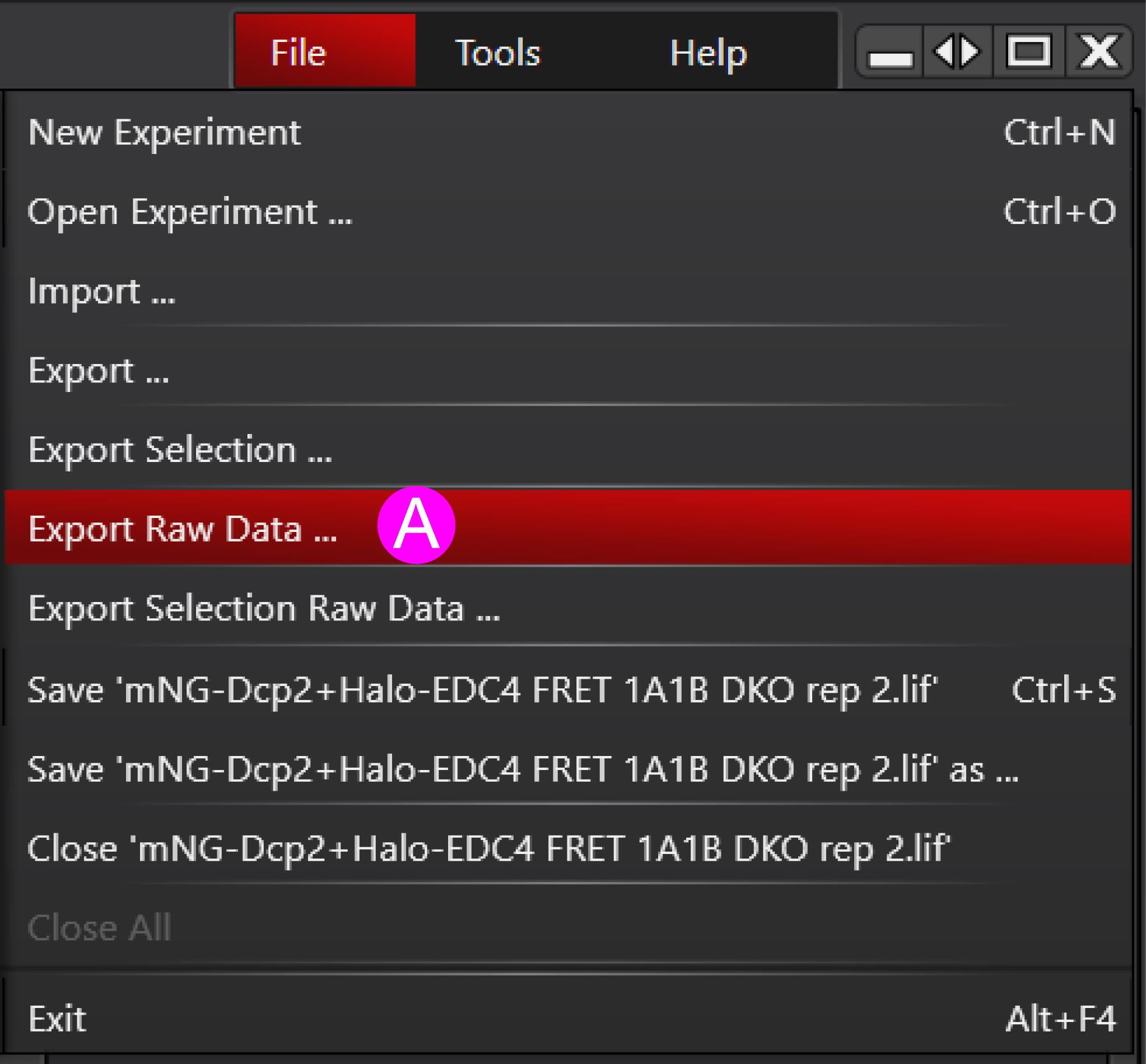
Figure 6. File menu for exporting raw fluorescence lifetime imaging (FLIM) data. (A) Select Export Raw Data … from the drop-down menu at the top of the FLIM module window to export FLIM captures as a .bin file.
3. Save each individual image as a .bin file.
4. Find the autocalibration settings for each image by clicking on Calibration from the Phasor tab of the FALCON module (Figure 7).
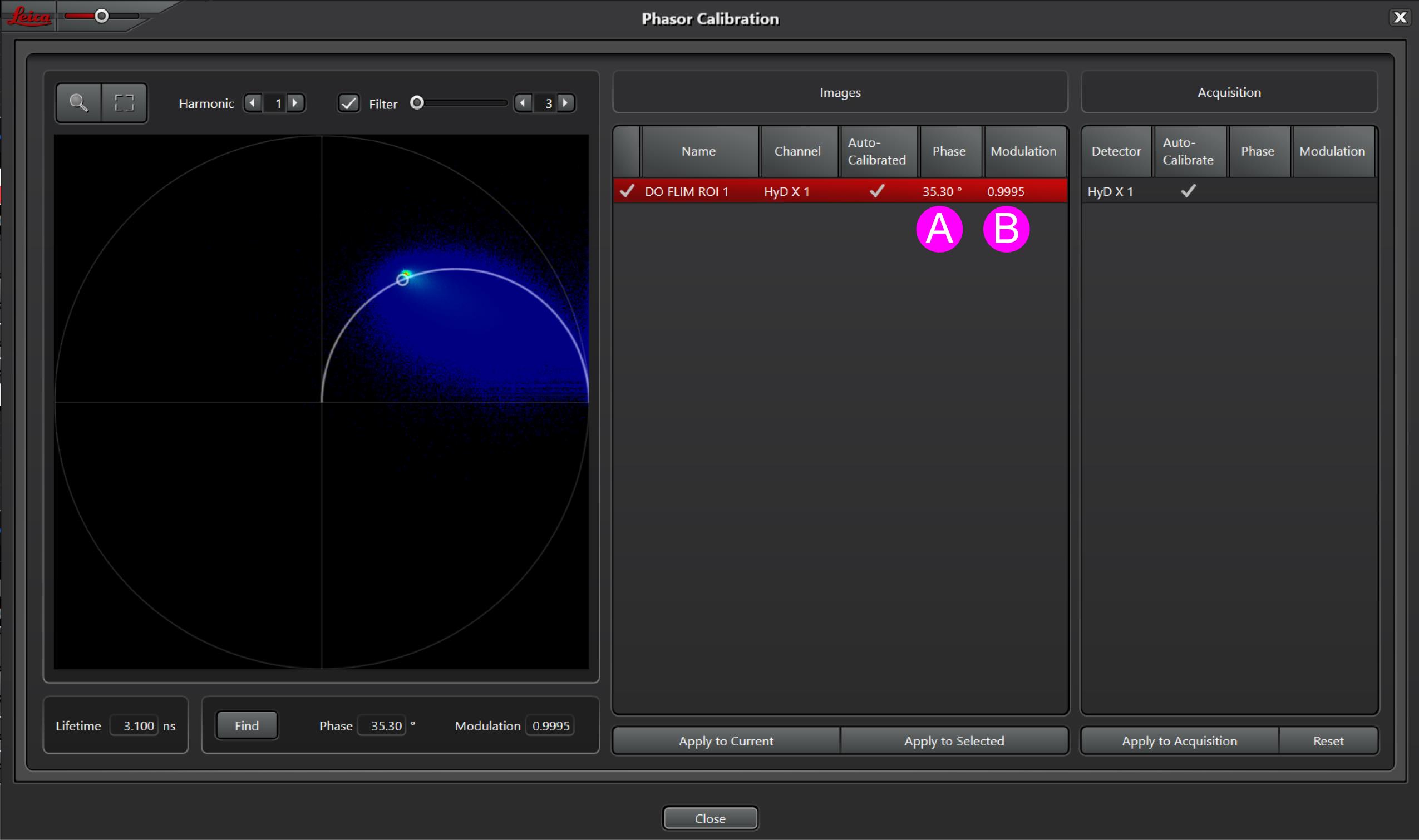
Figure 7. Fluorescence lifetime imaging (FLIM) calibration window. Autocalibration parameters for each FLIM image are found in this window. (A) Phase angle in degrees. (B) Modulation value.
5. Make note of the values for phi and modulation for each image. This information is needed for data analysis.
Data analysis
This data analysis pipeline quantifies the average RNP condensate fluorescence lifetime in donor-only samples (τD) and donor + acceptor samples (τD+A) to calculate FRET efficiency. A general workflow is outlined in Figure 2. First, TCSPC data is transformed to produce a two-dimensional phasor plot. This phasor plot is then processed in two ways. The first applies a complex wavelet filter to resolve condensate-specific datapoints that are used to segment the condensed phase from dilute phase regions, generating a condensate-only image (MaskRNP). The second transformation excludes datapoints with low-confidence fluorescence lifetime calculations from the raw unfiltered phasor. This second transformation is then used to produce a fluorescence lifetime image (τphasor) containing high-confidence lifetime measurements only. See General note 5 for FLIM-FRET analysis of non-condensate proteins.
Each method of phasor data processing presents its own challenges. Complex wavelet filtering is an effective method to spatially separate pixels in the condensed phase from the surrounding dilute phase and autofluorescence. However, this method distorts phasor positions and therefore obscures fluorescence lifetime estimations. Unprocessed phasor-transformed TCSPC data can be used to calculate fluorescence lifetimes, but lack the spatial resolution necessary for image segmentation. To overcome the challenges of each approach, phasor-transformed TCSPC data are processed independently using both methods before integrating phasor segmentation and lifetime calculations to generate condensate-segmented FRET efficiency (Figure 2).
The Python code and data files needed for this data analysis protocol can be found at https://github.com/LeeLabBCM/ComplexWaveletFilter. Install the wavelet filtering analysis package from the GitHub repository and follow the installation instructions.
A. Processing raw .bin files for phasor transformation
For raw TCSPC data exported from LAS-X and .bin files, use the following steps to convert them to .tiff files.
1. Open .bin files in FIJI using the Bio-Formats plugin.
a. Navigate to Plugins > Bio-Formats > Bio-Formats importer and select a .bin file to import.
b. The open file should be a stack with 132 slices and contain the raw TCSPC data. Save this stack as a .tif file. This is the file you will import into FLUTE [25] for further processing.
Note: If files cannot be imported using FIJI, a Python script located in the GitHub repository for wavelet filtering analysis will convert single-channel .bin files exported from LASX into .tif files (see Data analysis, step B1).
Critical: .tif files need to be 32-bit for import into FLUTE. If the raw .bin file does not open as 32-bit, convert it in FIJI by navigating to Image > Type > 32-bit.
B. Phasor transformation of TCSPC data in .tiff format
1. Use FLUTE to transform the raw TCSPC data for phasor analysis. Follow the installation instructions found in the GitHub repository: https://github.com/LaboratoryOpticsBiosciences/FLUTE.
2. Set the calibration parameters for phasor transformation. FLUTE uses a TCSPC capture from a reference dye of known fluorescence lifetime to calibrate the phasor plot. The Leica Stellaris 8 FALCON has an autocalibration feature that uses the instrument response function (IRF) of the laser for calibration. Calibration values can be entered into FLUTE manually, but a calibration image is still needed to set the microscope capture settings.
a. From the main FLUTE window, select Load Calibration (Figure 8A).
b. Bin Width (ns) is the time interval between photon collection for the raw TCSPC data in nanoseconds, Laser Freq. (MHz) is the pulse frequency of the laser in MHz, Tau Ref. (ns) is the expected fluorescence lifetime of the reference dye in nanoseconds, and Harmonic is the harmonic used for phasor transformation. For a Leica Stellaris 8 FALCON using a 78 MHz laser, enter 0.097 and 78 in the sections for bin width and laser frequency, respectively. Keep Tau Ref. (ns) and Harmonic at 4.0 and 1.0, respectively.
c. Click the button Choose File and select the calibration reference file provided in the wavelet filtering GitHub repository.
d. In the main FLUTE window, numbers will propagate next to Phi Calibration: and M Calibration:, which represent the phase angle and modulation values, respectively. Manually enter the phi and modulation values found in LASX (Figure 8B–C). The phi value needs to be entered as a negative value of the phi angle in radians.
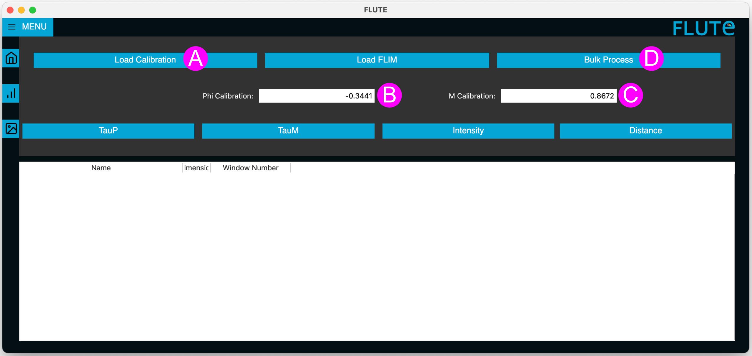
Figure 8. FLUTE user interface window. This is the main window for the FLUTE software package. (A) Button to open the calibration settings window. (B) Phase angle (phi) in radians. (C) Modulation value for phasor calibration settings. These values (A–C) can be changed manually to enter the autocalibration values from LASX. Alternatively, the values can be computed based on FLIM data from a reference dye of known fluorescence lifetime. (D) Button for generating phasor coordinate images.
e. A window will appear with options to enter the calibration parameters necessary for the phasor transformation (Figure 9).
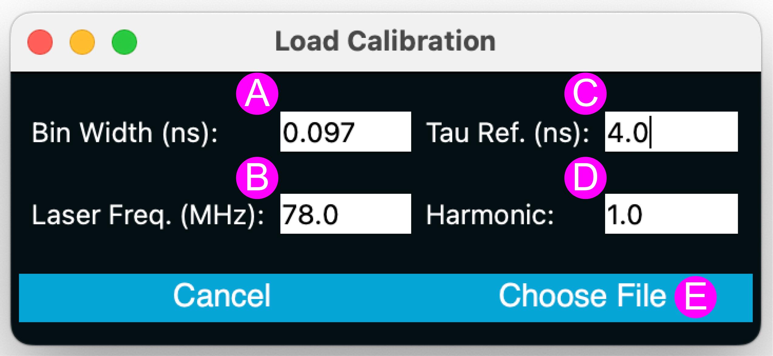
Figure 9. FLUTE calibration settings window. Window for entering FLIM system settings and reference dye information. (A) Location to enter the bin width of the exported TCSPC data. (B) Location to enter the frequency of the laser used to capture FLIM data. (C) Location to enter the expected fluorescence lifetime of the reference dye if calibrating using a reference dye FLIM image. (D) Harmonic for phasor transformation. (E) Button to load a reference dye FLIM image if used for calibration.
3. Import TCSPC .tif images into FLUTE and export the phasor coordinates. Select Bulk Process from the main FLUTE window. A file navigation menu will open. Navigate to your TCSPC .tif files saved from FIJI (see Data analysis, step A1b) and select files to process. Keep in mind that individual images will have different calibration values and need to be processed separately. If large tile scans were captured, each tile will have the same calibration value and can be processed together.
4. The G and S coordinate images generated in FLUTE are not in the correct OME-TIFF format required for downstream processing in Python. Convert the G and S coordinate images obtained from FLUTE to properly formatted .tiff files by opening them in ImageJ and saving over the original files.
5. Generate an intensity image from the TCSPC data by summing the photons collected at each pixel over time.
a. Open the .tiff file created in Data analysis, section A.
b. Navigate to Image > Stacks > Z-projection > Sum Slices and save this file as a .tif file.
Critical: This file is needed for wavelet filtering in Python in a later step of the analysis. Save it in a dedicated location.
6. After completion of these steps, the original .bin file will have been used to generate a G coordinate image, an S coordinate image, and an intensity image, which are all 32-bit .tiff files. These files can now be processed to generate wavelet-filtered and unfiltered phasors for segmentation and fluorescence lifetime analysis.
7. A new window will open to select the export location. Locate the files ending in _g.tiff and _s.tiff in the export location. These files and the intensity file created with FIJI will be used for the next step of the analysis.
Critical: Move the files ending in _g.tiff and _s.tiff to the location where their corresponding intensity image is saved (see Data analysis step B5).
C. Wavelet filtering
1. Install the wavelet filtering analysis package from the GitHub repository and follow the installation instructions (https://github.com/LeeLabBCM/ComplexWaveletFilter).
2. Run the ComplexWaveletFilter.py script to generate a wavelet-filtered dataset. The .tif files for intensity and phasor coordinates (files ending in _g.tiff and _s.tiff) should be located in the same folder. Select the folder when prompted by the Python script.
3. Input the transformation harmonic, the expected lifetime of the fluorophore that was imaged, and the wavelet filtering level. The harmonic should be the value entered in FLUTE to generate unfiltered phasor coordinates. The fluorophore used for the sample data provided is mNeonGreen with an expected lifetime of 3.1 ns. The sample dataset should use 9 filter levels. If the expected lifetime of a fluorophore is unknown, use the phasor module in LASX to estimate its fluorescence lifetime.
4. The output for the ComplexWaveletFilter.py script is two compressed files ending with .npz in a folder called “datasets.” One file will have “CWF” in the file name, containing wavelet-filtered phasor coordinates that will be used for RNP condensate segmentation. The other file will have “unfiltered” in the file name and will be used for lifetime calculation. Phasor plots generated from wavelet-filtered data can be seen in Figure 10.
Note: Wavelet filtering levels affect the separation between condensed and dilute phase phasor clusters. More filtering levels will increase separation between the two clusters, but it also distorts the phasor position. This interferes with the segmentation strategy that uses the expected lifetime of the FRET donor fluorophore to guide the automated approach (see Data analysis, step D3). Better separation may be achieved by increasing the filter levels. In this case, it may also be necessary to increase the size of the ROI radius.
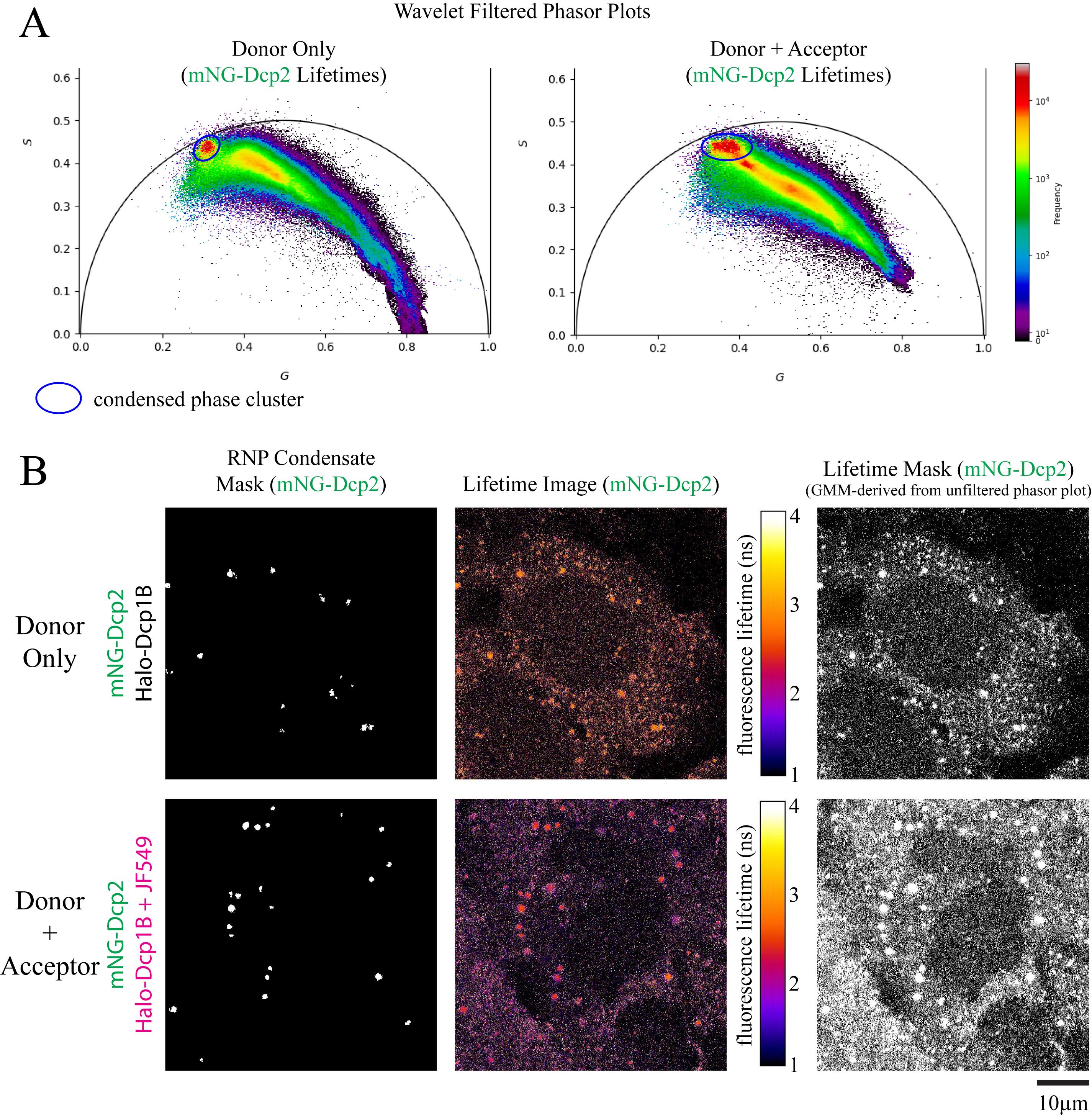
Figure 10. Python script analysis output. Representative output data from the referenced GitHub repository. (A) Wavelet filtered phasor plots created by CondensedPhaseGMM.py. The blue ellipse marks the ROI placement from the Gaussian mixture model (GMM) for the condensed phase cluster. Data from mNG-Dcp2 (donor only) and mNG-Dcp2 plus Halo-Dcp1B conjugated to JF549 (donor + acceptor). Dcp2 and Dcp1B are two known decapping complex interaction partners. (B) Images created by CondensedPhaseGMM.py and Circular_ROI_lifetime.py. Ribonucleoprotein (RNP) condensate masks are created by CondensedPhaseGMM.py and correspond to pixels that fall within the blue elliptical regions of interest (ROIs) from panel A. Lifetime images and lifetime masks are created by Circular_ROI_lifetime.py. The lifetime images for the donor only and donor + acceptor captures contain lifetime values for pixels that fall inside unfiltered phasor ROIs. Scale bar = 10 µm.
D. Automated segmentation of the wavelet-filtered phasor to generate the RNP condensate mask
For condensed phase segmentation, the complex wavelet filter reveals a condensed phase cluster that is spatially distinct from the dilute phase and autofluorescence signals. This separation is defined by the presence of condensed phase pixels along the universal circle, with dilute phase pixels residing within the circle.
Note: For condensates with lower partitioning, the distance between condensed and dilute phase clusters is smaller than for condensates with high partitioning. See Troubleshooting 2 and 3.
We use an automated approach to define a region of interest around the condensed phase cluster. First, a GMM is applied to the wavelet-filtered phasor plot to locate the center of the condensed phase cluster. Next, an elliptical ROI is drawn around the condensed phase cluster, with its major and minor axis lengths and rotation angle defined by the magnitudes and directions of the GMM covariance eigenvectors. These computations are performed by the CondensedPhaseGMM.py script provided in the analysis package. This segmentation approach has been previously validated and benchmarked against standard, intensity-based segmentation and was found to detect more granules than current standard methods [15] (Figure 11).
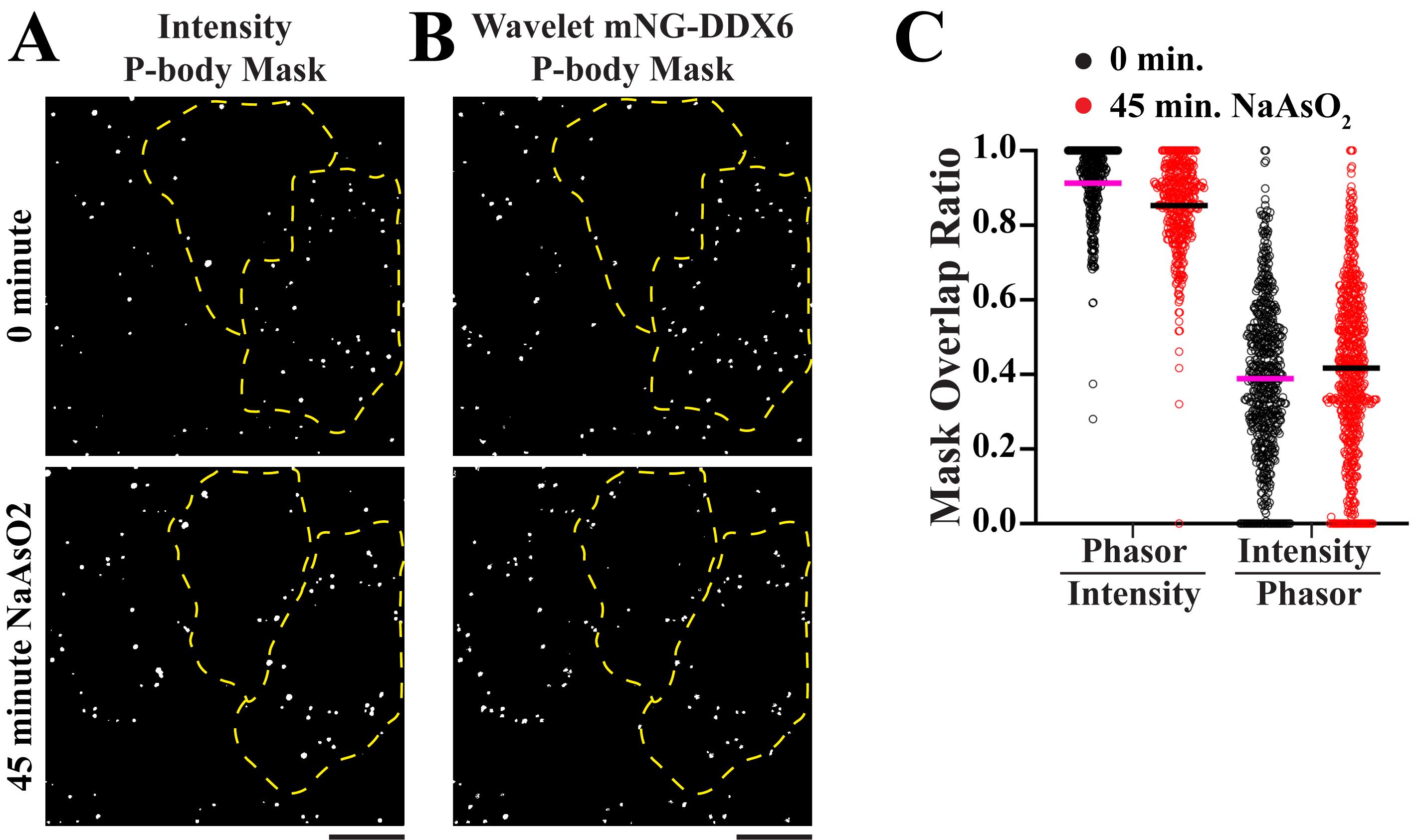
Figure 11. Benchmarking phasor segmentation against intensity-based segmentation. Data from [15]. (A) Representative masks of P-bodies labeled with the marker mNeonGreen-DDX6 generated using intensity-based thresholding before and after 45 min of NaAsO2 stress (500 μM). (B) Representative masks of P-bodies labeled with the marker mNeonGreen-DDX6 generated using phasor-based lifetime thresholding before and after 45 min of NaAsO2 stress (500 μM). Yellow outline denotes cell boundaries. Scale bars = 10 μm. (C) Performance of phasor segmentation compared to intensity segmentation was quantified by overlaying the two masks and computing their overlap. Magenta and black lines indicate the mean mask overlap ratio across three independent biological replicates. Phasor-segmentation outperformed intensity segmentation via increased sensitivity for detecting more granules. N = 3 biological replicates, n = 91 cells.
1. Run the CondensedPhaseGMM.py script and select the wavelet-filtered .npz file generated with the ComplexWaveletFilter.py script. Enter the same harmonic and fluorescence lifetime value entered for the ComplexWaveletFilter.py script when prompted.
2. Prompts will ask for a multiplication factor and a shift factor. The program will determine the radius of a segmentation ROI proportional to the coefficient of variance at the center of the condensed phase cluster. Enter a value greater than 1 to increase the size of the ROI or less than 1 to decrease the size. The distance on the phasor plot between the condensed phase cluster and the dilute phase cluster is proportional to the partition coefficient of the RNP protein being imaged. For proteins with low partition coefficients, the condensed phase ROI can pick up dilute phase pixels. To account for this, we provide the option to include a shift factor that moves the ROI position away from the dilute phase cluster. Enter a value greater than zero to shift the ROI position or enter zero for no shift.
3. Enter a radius to filter the dataset for GMM cluster identification in phasor units when prompted. A radius of 0.1 is sufficient to identify the center of the condensed phase cluster for the sample dataset, but should be empirically determined for each type of RNP being analyzed.
4. The output for the CondensedPhaseGMM.py script is a binary mask called “ellipse_mask.tiff” located in a folder called “mask,” and a phasor plot located in a folder called “phasor” (Figure 10A).
Note: The values provided are a starting point for segmentation and may need to be adjusted based on the samples being analyzed. If the resultant mask does not encompass all bright foci in the field, increase the multiplication factor or increase the radius of the GMM. If the resultant mask is detecting regions outside of condensate foci (i.e., dilute phase), try reducing the multiplication factor or GMM radius. If the condensate being analyzed has a low partition coefficient (causing poor separation between dilute and condensed phase clusters), include a shift factor that will move the GMM further from the dilute phase clusters or increase the filtering levels.
E. Generation of segmented lifetime image from unfiltered phasor
Fluorescence lifetime calculation accuracy is highly dependent on photon counts for lifetime data in the time domain (TCSPC data) and frequency domain (phasor transformation). A common approach to estimating fluorescence lifetime for every pixel in an image is by combining photon counts from neighboring pixels and assigning the median phasor coordinate values. This method cannot be used for calculating fluorescence lifetime in condensates because photons from proteins in the condensed and dilute phases would be combined for lifetime calculations. For RNP FLIM-FRET analysis, we use an alternative approach that excludes low-confidence pixels from the analysis by defining a region of interest around the highest density center of the phasor data. To implement this, a GMM is used to locate the center of the unfiltered phasor data before applying a ROI proportional to the variance around the phasor’s Gaussian center. From this, a lifetime image containing only pixels that correspond to points inside the unfiltered phasor ROI is generated. This method effectively excludes lifetime values on the basis of lifetime confidence and not intensity or a lifetime estimate that includes undesired pixels. The condensed phase mask and the processed lifetime image are then combined to calculate an average fluorescence lifetime within RNP condensates.
1. Run the Circular_ROI_lifetime.py script and select the unfiltered .npz file when prompted.
2. The output will be two .tiff files located in a folder called “unfiltered_lifetime.” The file with “mask” in the name is a binary mask indicating pixel locations with high-confidence lifetime calculations. The file with “lifetime” in the name is the unfiltered lifetime image (Figure 11B).
F. Processing of masks and lifetime images in ImageJ
1. Open the RNP condensate mask located in the “mask” folder in ImageJ.
2. Select Set Measurements > Integrated Density.
3. Convert the wavelet-generated mask to an 8-bit image. Select Image > Type > 8-bit.
4. Generate ROIs for all condensates within the mask.
a. Select Analyze > Analyze Particles.
b. Choose a size range for condensates that corresponds to cell type and zoom factor. For U2OS cells captured with a 5× zoom factor, the size range of 20-Infinity eliminates any smaller cytosolic structures or out-of-focus P-bodies within the mask.
5. Close the wavelet-generated mask and open the binary mask generated from the unfiltered phasor in ImageJ (.tiff file with “mask” in the file name located in the “unfiltered_lifetime” folder).
6. Select all ROIs within the ROI manager and click measure. Then, copy this data into an Excel spreadsheet.
7. Close the binary mask generated from the unfiltered phasor and open the corresponding lifetime image (.tiff file with “lifetime” in the file name located in the “unfiltered_lifetime” folder).
8. Select all ROIs within the ROI manager, click measure, and copy this data into the Excel spreadsheet.
9. Repeat this process for both the donor-only and donor + acceptor images.
G. Calculating FRET efficiency
1. Divide the integrated density measurements from the lifetime image by the integrated density measurements from the binary mask to obtain a per-granule lifetime value. Repeat this step for both the donor-only and donor + acceptor values.
2. Once a list of condensate lifetimes has been obtained for the donor-only image, calculate the average lifetime from this population.
3. Calculate the FRET efficiency per granule using the following equation: EFRET = 100 · [1-(τD+A/τD)].
a. τD = average donor-only lifetime, calculated in the previous step.
b. τD+A = each individual donor + acceptor lifetime value, calculated by dividing the integrated density of each ROI within the lifetime image by the integrated density of the corresponding ROIs in the binary mask.
Note: Since the donor-only value is derived from a single point on the phasor, error can be reduced from this measurement by increasing the number of donor-only cells captured. Furthermore, instead of computing the FRET efficiencies on a per-granule basis, a similar computation can be performed on the donor + acceptor data, with only the center point of the donor + acceptor phasor plot being used in the FRET efficiency lifetime calculation for a particular image. This can reduce the overall error due to the increased number of cells and pixels being sampled per lifetime measurement.
4. Statistical comparisons:
a. At least three biological replicates are recommended per experiment, with donor-only and donor + acceptor measurements captured under the same conditions, during the same acquisition session.
b. This method analyzes all granules in a given field, meaning FRET efficiency values can be reported as an average FRET efficiency per granule, per cell, or per field of view (see General note 6).
c. FRET efficiencies can be statistically compared across different conditions (e.g., before and after stress) using standard statistical methods (e.g., t-test, ANOVA).
Validation of protocol
This protocol has been used and validated for detecting interactions in several different mRNA processing body factors (Dcp2-Dcp1A, DDX6-Lsm14a as a positive control, and Dcp2-DDX6 as a negative control) (Figure 12). These experiments can be found in the following article:
Fahim et al. [15]. Fluorescence lifetime sorting reveals tunable enzyme interactions within cytoplasmic condensates. J Cell Biol.
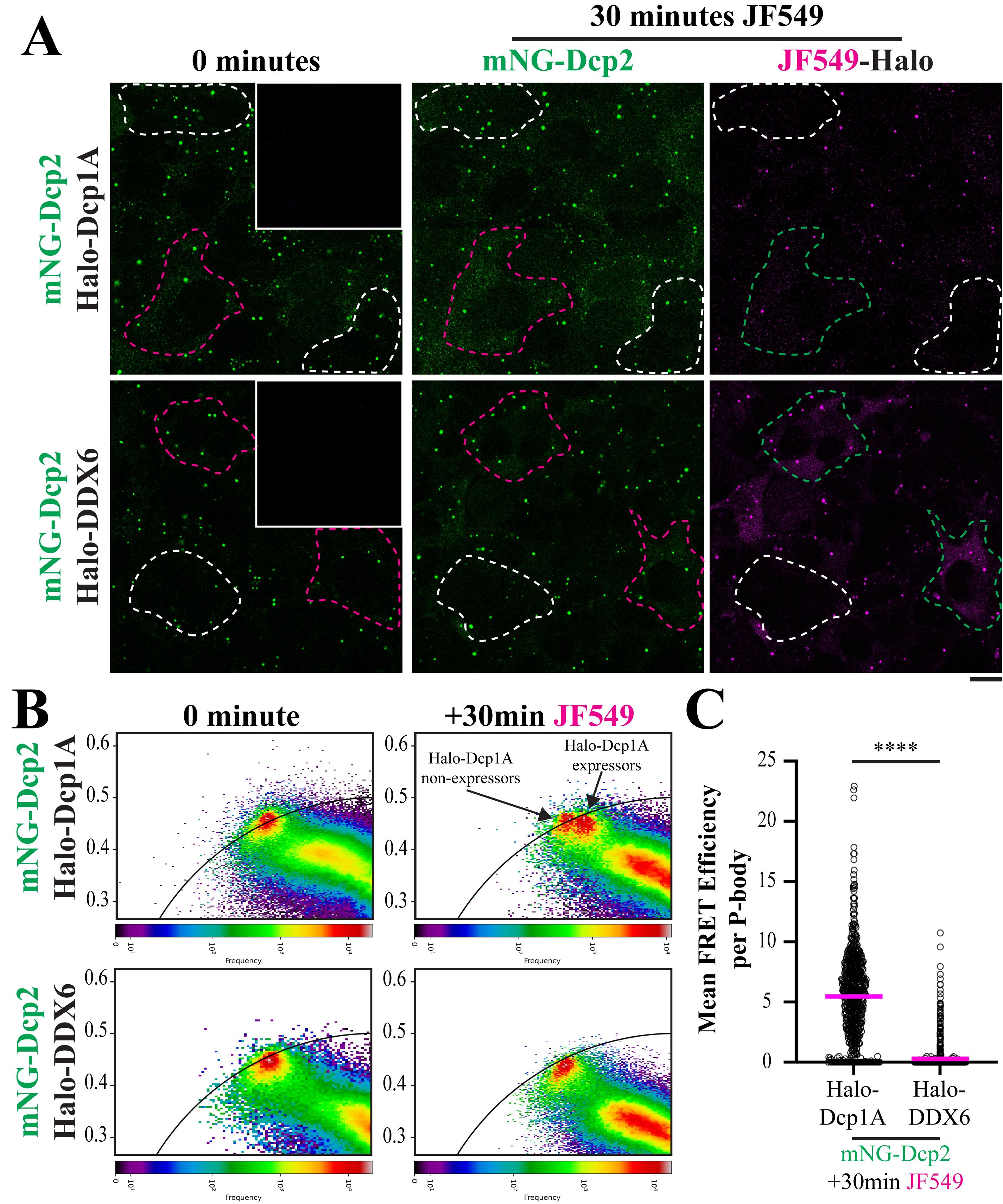
Figure 12. Representative fluorescence lifetime imaging–Forster resonant energy transfer (FLIM-FRET) data between the P-body-localized mRNA decapping factors. Data from [15]. (A) Representative images of U-2 OS cells expressing mNG-Dcp2 (FRET donor) and Halo-Dcp1A (FRET acceptor) or mNG-Dcp2 and Halo-DDX6. FLIM images were captured of the same cells before (donor-only) and after the addition of Janelia Fluor (JF)-549 (donor + acceptor) for 30 min. White outlines indicate cells that do not express Halo-Dcp1A or Halo-DDX6, and green/magenta outlines indicate cells expressing these Halo constructs. Scale bar = 10 μm. (B) Representative phasors before and after the addition of JF549. (C) FRET efficiency calculation for the interaction between two known decapping complex interaction partners (Dcp2 and Dcp1A) within P-bodies and two known non-interacting P-body factors (Dcp2 and DDX6). The magenta lines indicate the mean FRET efficiency within P-bodies across three independent biological replicates. Significance was determined by a nested T test. ****P < 0.00001. n = 133 and 109 cells in Halo-Dcp1A- and Halo-DDX6-expressing cells across three biological replicates, respectively.
General notes and troubleshooting
General notes
1. This protocol is amenable to the use of different fluorescent molecules as FRET pairs. When selecting molecules, ensure the emission spectrum of the donor partially overlaps with the excitation spectrum of the chosen acceptor. A useful tool to visualize and test these spectra can be found here: https://www.fpbase.org/fret. Additionally, the brightness of the donor fluorophore must be sufficiently high to yield a suitable amount of signal (>100 photons per laser pulse). Since FRET involves a transfer of energy from the donor to the acceptor, expect a decrease in donor intensity in cases of strong FRET.
2. The maximum fluorescence lifetime that can be accurately measured is determined by the laser frequency. Incomplete decay curves result in inaccurate decay curve fitting and, therefore, inaccurate fluorescence lifetime calculation. Generally, with a high repetition rate laser, like the 78 MHz laser used in this protocol, fluorophores with fluorescence lifetime <4 ns can be measured with high enough accuracy to interpret bulk changes in fluorescence lifetime due to FRET. However, this should be considered when interpreting small changes in fluorescent lifetime.
3. This protocol uses HaloTag in conjunction with a cell-permeable acceptor ligand to capture both reference donor lifetime and experimental donor–acceptor lifetime within the same cell line. However, other chemical handles, such as SNAPtag, may also be used. Furthermore, if these chemical handles are unavailable, a similar result can be achieved with constitutively fluorescent molecules (e.g., mNeonGreen and mScarlet). For this approach, generate one cell line that only expresses the donor fluorescent protein and capture data to use as the reference lifetime. Then, generate a cell line expressing both donor and acceptor fluorescent proteins to capture donor–acceptor experimental lifetimes.
4. During acquisition, cross-excitation of the acceptor fluorophore can occur, resulting in artificially longer or shorter lifetime values, depending on the lifetime of the acceptor. To mitigate this, lower the donor excitation laser wavelength and shorten the donor detector window size to avoid cross-excitation or incidental detection of the acceptor fluorophore.
5. This protocol can be implemented to analyze FLIM-FRET between non-condensate proteins. Experimental design and data acquisition steps remain the same. However, depending on the localization of the protein of interest, segmentation may or may not be necessary. Included is an example of FLIM-FRET between the endoplasmic reticulum (ER) proteins Lsg1 and VAPB (Figure 2A). Here, since the donor localizes exclusively to the ER, segmentation is not required, and unfiltered lifetime values are all that is needed. Alternatively, if the donor’s localization is not within a condensate and can be segmented using more traditional means (e.g., fluorescence intensity–based thresholding methods), then this can be used in place of the wavelet-filtered condensate segmentation. For this application, the wavelet-filtering method to generate MaskRNP is omitted, and τphasor is used directly for FRET analysis or with an alternative binary mask.
6. The size of analyzable granules will be determined by the maximal resolution of the system being used. If particles of interest are represented by very few pixels, it may be necessary to compute FRET efficiencies on a per-cell or per-field basis to reduce error. Alternatively, the center of the donor + acceptor phasor can be used as a single lifetime measurement for the entire field of view.
7. An update to LASX software (version 4.0 and newer) exports TCSPC .bin files separated by channel. If using a newer version of LASX, it is not necessary to capture the single channel as instructed in section C3 of the procedure. All .bin files exported from LASX version 4.0 and newer will be in the correct format for the data analysis workflow.
8. For FLIM platforms that acquire fluorescence lifetime data directly in the frequency domain, phasors can be independently propagated using the phase shift and modulation values captured directly in these systems. G and S phasor coordinates can be computed for each pixel [22]:
G = m * cos(phi)
S= m * sin(phi)
Where m is the modulation and phi is the phase shift. Frequency domain system users can generate .tiff files of computed G and S phasor coordinates and intensity values as input for the Python scripts (section C of data analysis).
Troubleshooting
1. Low photon counts/fluorescence signal: If the particular condensate protein being imaged does not yield a sufficient number of photons within the condensate, the following acquisition settings can be adjusted to increase signal: Increase the excitation laser power, reduce the scan speed, decrease the pixel format, or increase the number of line accumulations. If this still does not elevate the signal enough, consider using a brighter donor fluorophore (e.g., mNeonGreen).
2. Poor phasor segmentation: Phasor-based segmentation of the condensate cluster relies on clear separation from the dilute phase cluster. Different condensate proteins will exhibit varying degrees of separation depending on the brightness of the marker being used and the partitioning of the condensate factor. If the GMM does not effectively detect the condensed phase cluster, the following parameters can be adjusted to improve detection of the condensate cluster: Introduce a shift factor to move the identified cluster outward away from the dilute phase. Reduce the radius of the GMM or the multiplication factor to eliminate the detection of nearby dilute phase pixels. Increase the wavelet filtering levels. These modifications can be iteratively adjusted by viewing the resultant condensate mask after each adjustment to ensure that excess pixels outside of the desired condensate are not included in the final mask.
3. Low condensate protein partitioning: Some condensate factors have low partition coefficients, decreasing the separation between dilute and condensed phase clusters on the phasor. If this separation is too subtle for effective phasor-based condensed phase cluster discrimination, standard intensity-based segmentation can be used in lieu of wavelet-based phasor segmentation. All other steps of the analysis pipeline can be maintained.
Acknowledgments
Writing—Original draft, N.D.P., L.E.F.; Writing—Review & Editing: N.D.P., J.M.M., L.E.F., J.E.L.; Funding acquisition, J.E.L.; Supervision, J.E.L. This work was funded by the CPRIT Recruitment of First-Time, Tenure-Track Faculty Award (RR200065) (J.E.L.), the National Institutes of Health (NIH R35GM151054) (J.E.L.), and training fellowships from the Gulf Coast Consortia on the Training in Precision Environmental Health Sciences (TPEHS) (NIH grant T32ES027801) (N.D.P. and J.M.M.). This method was originally developed and validated in [15].
Competing interests
The authors declare no conflicts of interest.
References
- Li, P., Banjade, S., Cheng, H. C., Kim, S., Chen, B., Guo, L., Llaguno, M., Hollingsworth, J. V., King, D. S., Banani, S. F., et al. (2012). Phase transitions in the assembly of multivalent signalling proteins. Nature. 483(7389): 336–340. https://doi.org/10.1038/nature10879
- Keber, F. C., Nguyen, T., Mariossi, A., Brangwynne, C. P. and Wühr, M. (2024). Evidence for widespread cytoplasmic structuring into mesoscale condensates. Nat Cell Biol. 26(3): 346–352. https://doi.org/10.1038/s41556-024-01363-5
- Alberti, S. and Hyman, A. A. (2021). Biomolecular condensates at the nexus of cellular stress, protein aggregation disease and ageing. Nat Rev Mol Cell Biol. 22(3): 196–213. https://doi.org/10.1038/s41580-020-00326-6
- Hubstenberger, A., Courel, M., Bénard, M., Souquere, S., Ernoult-Lange, M., Chouaib, R., Yi, Z., Morlot, J. B., Munier, A., Fradet, M., et al. (2017). P-Body Purification Reveals the Condensation of Repressed mRNA Regulons. Mol Cell. 68(1): 144–157.e5. https://doi.org/10.1016/j.molcel.2017.09.003
- Jain, S., Wheeler, J. R., Walters, R. W., Agrawal, A., Barsic, A. and Parker, R. (2016). ATPase-Modulated Stress Granules Contain a Diverse Proteome and Substructure. Cell. 164(3): 487–498. https://doi.org/10.1016/j.cell.2015.12.038
- Kodali, S., Proietti, L., Valcarcel, G., López-Rubio, A. V., Pessina, P., Eder, T., Shi, J., Jen, A., Lupión-Garcia, N., Starner, A. C., et al. (2024). RNA sequestration in P-bodies sustains myeloid leukaemia. Nat Cell Biol. 26(10): 1745–1758. https://doi.org/10.1038/s41556-024-01489-6
- Currie, S. L., Xing, W., Muhlrad, D., Decker, C. J., Parker, R. and Rosen, M. K. (2023). Quantitative reconstitution of yeast RNA processing bodies. Proc Natl Acad Sci USA. 120(14): e2214064120. https://doi.org/10.1073/pnas.2214064120
- Tibble, R. W., Depaix, A., Kowalska, J., Jemielity, J. and Gross, J. D. (2021). Biomolecular condensates amplify mRNA decapping by biasing enzyme conformation. Nat Chem Biol. 17(5): 615–623. https://doi.org/10.1038/s41589-021-00774-x
- Padrón, A., Iwasaki, S. and Ingolia, N. T. (2019). Proximity RNA Labeling by APEX-Seq Reveals the Organization of Translation Initiation Complexes and Repressive RNA Granules. Mol Cell. 75(4): 875–887.e5. https://doi.org/10.1016/j.molcel.2019.07.030
- Pietraszewska-Bogiel, A. and Gadella, T. (2010). FRET microscopy: from principle to routine technology in cell biology. J Microsc. 241(2): 111–118. https://doi.org/10.1111/j.1365-2818.2010.03437.x
- Zeug, A., Woehler, A., Neher, E. and Ponimaskin, E. G. (2012). Quantitative Intensity-Based FRET Approaches—A Comparative Snapshot. Biophys J. 103(9): 1821–1827. https://doi.org/10.1016/j.bpj.2012.09.031
- Castellani, C. M., Torres-Ocampo, A. P., Breffke, J., White, A. B., Chambers, J. J., Stratton, M. M. and Maresca, T. J. (2020). Live-cell FLIM-FRET using a commercially available system. Methods Cell Biol. 158: 63–89. https://doi.org/10.1016/bs.mcb.2020.02.002
- Lin, H., Herman, P. and Lakowicz, J. R. (2003). Fluorescence lifetime‐resolved pH imaging of living cells. Cytometry Part A. 52(2): 77–89. https://doi.org/10.1002/cyto.a.10028
- Mangiarotti, A., Siri, M., Tam, N. W., Zhao, Z., Malacrida, L. and Dimova, R. (2023). Biomolecular condensates modulate membrane lipid packing and hydration. Nat Commun. 14(1): 6081. https://doi.org/10.1038/s41467-023-41709-5
- Fahim, L. E., Marcus, J. M., Powell, N. D., Ralston, Z. A., Walgamotte, K., Perego, E., Vicidomini, G., Rossetta, A. and Lee, J. E. (2024). Fluorescence lifetime sorting reveals tunable enzyme interactions within cytoplasmic condensates. J Cell Biol. 224(1): e202311105. https://doi.org/10.1083/jcb.202311105
- Perego, E., Zappone, S., Castagnetti, F., Mariani, D., Vitiello, E., Rupert, J., Zacco, E., Tartaglia, G. G., Bozzoni, I., Slenders, E., et al. (2023). Single-photon microscopy to study biomolecular condensates. Nat Commun. 14(1): 8224. https://doi.org/10.1038/s41467-023-43969-7
- Pliss, A., Levchenko, S. M., Liu, L., Peng, X., Ohulchanskyy, T. Y., Roy, I., Kuzmin, A. N., Qu, J. and Prasad, P. N. (2019). Cycles of protein condensation and discharge in nuclear organelles studied by fluorescence lifetime imaging. Nat Commun. 10(1): 455. https://doi.org/10.1038/s41467-019-08354-3
- Kapoor, A., Didier, P., Faivre, C., Frey, C., Hener, P., Stefan, T., Lequeu, T., Réal, E., Klymchenko, A., Anton, N., et al. (2026). Fluorescence based microviscosity mapping in membraneless organelles. bioRxiv. e697638. https://doi.org/10.64898/2026.01.05.697638
- Liu, Y., Mathew, L., Yu, C., Fu, L., Shu, Z., Kapoor, S. and Duan, M. (2024). The Molecular Mechanism of Fluorescence Lifetime of Fluorescent Probes in Cell Membranes. J Phys Chem Lett. 15(50): 12293–12300. https://doi.org/10.1021/acs.jpclett.4c02731
- Poojari, C., Wilkosz, N., Lira, R. B., Dimova, R., Jurkiewicz, P., Petka, R., Kepczynski, M. and Róg, T. (2019). Behavior of the DPH fluorescence probe in membranes perturbed by drugs. Chem Phys Lipids. 223: 104784. https://doi.org/10.1016/j.chemphyslip.2019.104784
- Watanabe, N., Suga, K., Slotte, J. P., Nyholm, T. K. M. and Umakoshi, H. (2019). Lipid-Surrounding Water Molecules Probed by Time-Resolved Emission Spectra of Laurdan. Langmuir. 35(20): 6762–6770. https://doi.org/10.1021/acs.langmuir.9b00303
- Ranjit, S., Malacrida, L., Jameson, D. M. and Gratton, E. (2018). Fit-free analysis of fluorescence lifetime imaging data using the phasor approach. Nat Protoc. 13(9): 1979–2004. https://doi.org/10.1038/s41596-018-0026-5
- Vallmitjana, A., Torrado, B. and Gratton, E. (2021). Phasor-based image segmentation: machine learning clustering techniques. Biomed Opt Express. 12(6): 3410. https://doi.org/10.1364/boe.422766
- Wang, P., Hecht, F., Ossato, G., Tille, S., Fraser, S. E. and Junge, J. A. (2021). Complex wavelet filter improves FLIM phasors for photon starved imaging experiments. Biomed Opt Express. 12(6): 3463. https://doi.org/10.1364/boe.420953
- Gottlieb, D., Asadipour, B., Kostina, P., Ung, T. P. L. and Stringari, C. (2023). FLUTE: A Python GUI for interactive phasor analysis of FLIM data. Biol Imaging. 3: e1017/s2633903x23000211. https://doi.org/10.1017/s2633903x23000211
Article Information
Publication history
Received: Apr 30, 2026
Accepted: Jun 21, 2026
Available online: Jul 9, 2026
Published: Aug 5, 2026
Copyright
© 2026 The Author(s); This is an open access article under the CC BY-NC license (https://creativecommons.org/licenses/by-nc/4.0/).
How to cite
Readers should cite both the Bio-protocol article and the original research article where this protocol was used:
- Powell, N. D., Marcus, J. M., Fahim, L. E. and Lee, J. E. (2026). Automated FLIM-FRET Segmentation Within RNP Condensates. Bio-protocol 16(15): e5775. DOI: 10.21769/BioProtoc.5775.
- Fahim, L. E., Marcus, J. M., Powell, N. D., Ralston, Z. A., Walgamotte, K., Perego, E., Vicidomini, G., Rossetta, A. and Lee, J. E. (2024). Fluorescence lifetime sorting reveals tunable enzyme interactions within cytoplasmic condensates. J Cell Biol. 224(1): e202311105. https://doi.org/10.1083/jcb.202311105

 Download Citation in RIS Format
Category
Cell Biology > Cell imaging > Live-cell imaging
Cell Biology > Cell imaging > Fluorescence
Biochemistry > Protein > Interaction > Protein-protein interaction
Do you have any questions about this protocol?
Post your question to gather feedback from the community. We will also invite the authors of this article to respond.
 Post a Question


