


- Protocols

- Articles and Issues
- For Authors
- About
- Become a Reviewer


Dual Color tau-STED Super Resolution Microscopy in Arabidopsis Root Tip


Published: Vol 16, Iss 15, Aug 5, 2026 DOI: 10.21769/BioProtoc.5774 Views: 287
Reviewed by: Subash Chandra GodarAnonymous reviewer(s)
 PDF
PDF  Ask a question
Original research article
The authors used this protocol in:

Mar 2025

Protocol Collections
Comprehensive collections of detailed, peer-reviewed protocols focusing on specific topics




Related protocols
Abstract
Super-resolution microscopy has transformed our ability to visualize subcellular structures, but its application in plant biology remains challenging due to the optical complexity of plant tissues. Here, we present a detailed protocol for tau-STED microscopy (Leica Microsystems), which combines stimulated emission depletion (STED) with fluorescence lifetime imaging (FLIM) to achieve nanoscale resolution while minimizing phototoxicity. This method leverages time-correlated single-photon counting (TCSPC) to separate fluorescence signals based on their lifetimes, enhancing signal specificity and enabling the visualization of elusive subcellular compartments in Arabidopsis thaliana root tips. The protocol covers sample preparation, fluorophore selection, microscope configuration, image acquisition, and data analysis, providing a step-by-step guide to optimize tau-STED imaging for plant cell biology. By addressing the unique challenges of plant tissue imaging, such as autofluorescence, refractive index mismatches, and light scattering, this approach facilitates super-resolution imaging of intracellular structures, including the plant endoplasmic reticulum–Golgi intermediate compartment (ERGIC). This protocol is designed to be accessible to researchers with basic microscopy experience and offers a robust framework for exploring subcellular dynamics in plants with unprecedented detail.
Key features
• tau-STED integrates STED signals with fluorescence lifetime via phasor analysis at confocal speeds, enabling low-noise super-resolution imaging.
• Morphometry analysis workflow at super resolution.
Keywords: Cell biology Super-resolution microscopy
Plant biology
STED
Lifetime
tau-STED
Arabidopsis thaliana
Super-resolution microscopy
Plant biology
STED
Lifetime
tau-STED
Arabidopsis thaliana
Graphical overview
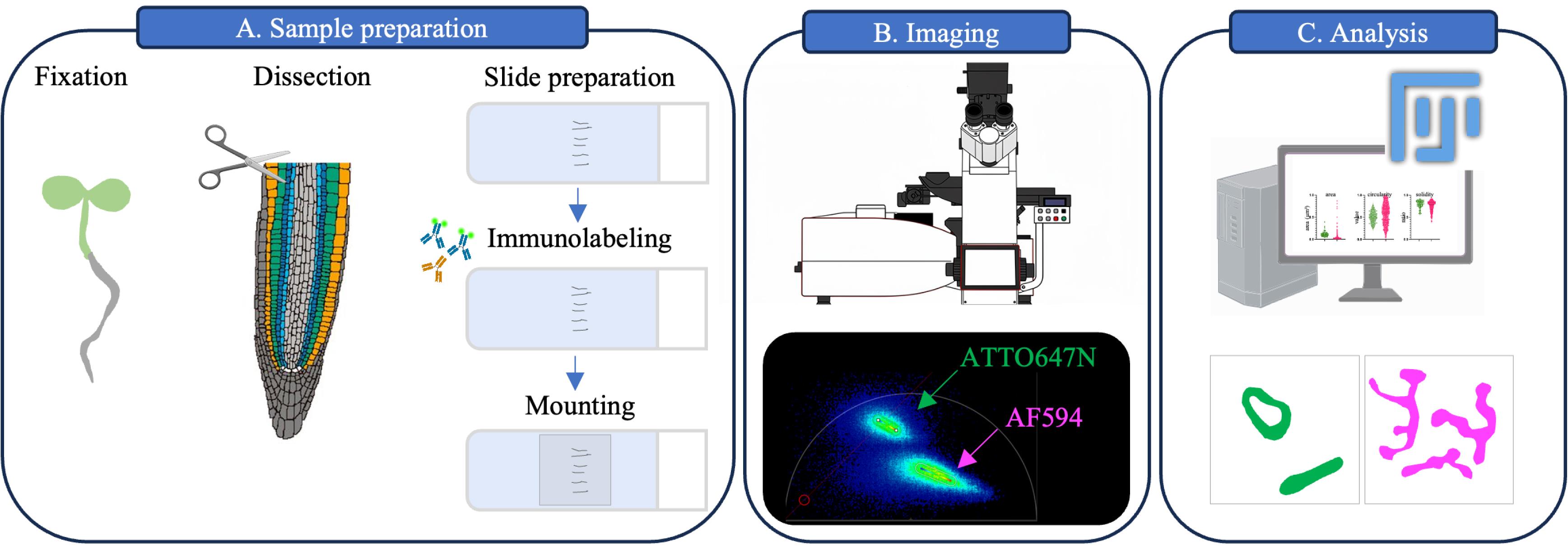
Schematic representation of the steps of the tau-STED microscopy in Arabidopsis root tips. (A) Sample preparation principal steps: chemical fixation, dissection of the root tip, slide preparation, immunolabeling, and mounting with MOWIOL. (B) Imaging of the sample using the SP8 STED FALCON after optimization. (C) Image analysis using FIJI.
Background
Super-resolution microscopy (SRM) has revolutionized the study of cellular processes by transcending the resolution limits of conventional light microscopy, achieving resolutions as fine as 10 nm in some cases. Techniques such as stimulated emission depletion (STED) and single-molecule localization microscopy (SMLM), both recognized by the 2014 Nobel Prize in Chemistry, have driven transformative biological discoveries by revealing subcellular details previously obscured by the diffraction barrier [1]. However, despite its immense potential, SRM remains underutilized in the study of cell wall–encapsulated organisms like plants, leaving a significant research frontier largely unexplored. This limited adoption stems from the intrinsic challenges posed by plant samples, including the rigid and complex structure of the cell wall, tissue heterogeneity, internal air spaces, and high levels of autofluorescence from pigments and secondary metabolites. These factors collectively complicate the application of SRM in plant biology, often obscuring the fine details of subcellular organization.
Among SRM techniques, STED microscopy stands out for its ability to surpass the diffraction limit of conventional fluorescence microscopy. By employing a depletion laser to selectively switch off fluorophores at the periphery of the excitation spot, STED achieves nanometer-scale resolution, enabling the visualization of subcellular structures with unprecedented clarity [1,2]. This depletion process not only refines spatial resolution but also alters the photophysical properties of fluorophores, particularly their fluorescence lifetime—the average time a fluorophore remains in the excited state before emitting a photon. As the depletion laser pushes fluorophores back to the ground state, it effectively shortens their lifetime, creating a distinction between depleted and non-depleted states [3,4]. However, STED has historically been less frequently applied to plant tissues due to two main challenges: the limited imaging depth of SRM objectives and the degradation of image quality caused by high background fluorescence emitted within the tissue under depletion. Consequently, it was long assumed that STED was not very efficient in plant tissues.
To fully exploit this lifetime information, Leica Microsystems developed tau-STED, an advanced technology that integrates STED with fluorescence lifetime imaging using time-correlated single-photon counting (TCSPC) [5–7]. During imaging, tau-STED simultaneously depletes the sample and collects photon lifetime data, accumulating information that allows fluorescence signals to be separated based on their distinct lifetimes. By filtering out background photons and by prioritizing photons from the doughnut center, tau-STED significantly improves resolution and enhances signal specificity, making it particularly effective for challenging samples like plant tissues. This innovation has opened new avenues for plant cell biologists, enabling the visualization of structures that were previously difficult to resolve.
One of the most compelling applications of tau-STED in plant biology is its ability to identify and characterize the plant endoplasmic reticulum–Golgi intermediate compartment (ERGIC) [8]. In our disruptive study [8], we employed tau-STED to distinguish the ERGIC from other membrane-bound compartments in Arabidopsis thaliana, uncovering its unique organization. The ERGIC’s close association with the endoplasmic reticulum and Golgi apparatus had long made it difficult to visualize using conventional microscopy. However, tau-STED’s capacity to resolve fine structural details and separate overlapping signals based on fluorescence lifetime proved instrumental in clarifying the ERGIC’s distinct identity and function. This discovery underscores tau-STED’s potential to reveal previously elusive subcellular structures, establishing it as an invaluable tool for investigating intracellular trafficking and organelle dynamics in plants.
Building on these advancements, this protocol offers a comprehensive, step-by-step guide to using tau-STED microscopy for visualizing subcellular compartments in Arabidopsis root tips. From sample preparation—including fixation, dissection, immunolabeling optimization, and fluorophore selection—to image acquisition and data analysis, each stage is designed to maximize resolution and signal quality while minimizing phototoxicity. By addressing the unique challenges of plant tissue imaging, this approach empowers researchers to explore the intricate subcellular landscapes of plants with unprecedented precision.
Materials and reagents
Biological materials
1. Arabidopsis thaliana transgenic fluorescent line pUBQ10::mCherry-MEMB12 and p35S::NAG-EGFP [9,10] or any relevant fluorescent transgenic line
Reagents
1. Distilled water
2. Murashige and Skoog medium (MS) (Duchefa Biochemie, catalog number: M0222.0050)
3. Sucrose (Sigma-Aldrich, catalog number: H4034-500G)
4. Plant agar (Duchefa Biochemie, catalog number: P1001.1000)
5. MES [2-(N-morpholino)ethanesulfonic acid] (Euromedex, catalog number: EU0033-A)
6. 1,4-piperazinediethanesulfonic acid (PIPES) (Sigma-Aldrich, catalog number: P6757-100G)
7. Ethylene glycol-bis(2-aminoethylether)-N,N,N′,N′-tetraacetic acid (EGTA) (Sigma-Aldrich, catalog number: E4378-100G)
8. Magnesium sulfate (MgSO4) (Euromedex, catalog number: P027-A)
9. Potassium hydroxide (KOH) (Sigma-Aldrich, catalog number: P5958-500G)
10. Paraformaldehyde (PFA) 16% (Ted Pella, catalog number: 18505)
11. Driselase (Sigma-Aldrich, catalog number: D9515-5G); store at -20 °C
12. Dimethyl sulfoxide (DMSO) (Sigma-Aldrich, catalog number: D8418-250ML)
13. IGEPAL CA-630 (Sigma-Aldrich, catalog number: I3021)
14. Normal donkey serum (NDS) (Abcam, catalog number: ab7475-10mL)
15. ChromoTek GFPboosterATTO647N (Proteintech, catalog number: gba647n)
16. ChromoTek RFPboosterATTO594 (Proteintech, catalog number: rba594)
17. FluoTag®-X4 anti-RFP abberior STAR 635P (Nanotag, catalog number: N0404-Ab635P-L)
18. Anti-MEMB (not commercially available [10])
19. Goat anti-rabbit IgG (H+L) cross-adsorbed secondary antibody, Alexa FluorTM 594 (Thermo Fisher Scientific, catalog number: A-11012)
20. Tris base (Sigma-Aldrich, catalog number: T6066)
21. Hydrochloric acid (HCl) 37% (Sigma-Aldrich, catalog number: 320331-2.5L)
22. Glycerol (Sigma-Aldrich, catalog number: G5516)
23. Mowiol 4-88 (Merck, catalog number: 475904)
24. 1.4-Diazabicyclo-2.2.29-octan (DABCO) (Sigma-Aldrich, catalog number: 27802)
Solutions
1. MES 0.5% pH 5.8 (see Recipes)
2. 1/2 Murashige and Skoog agar plate (1/2 MS agar plate) (see Recipes)
3. Microtubule Stabilizing Buffer 4/3 solution (MTSB 4/3 solution) (see Recipes)
4. Microtubule Stabilizing Buffer 1× solution (MTSB 1× solution) (see Recipes)
5. Fixation solution (see Recipes)
6. Cell wall digestion buffer (see Recipes)
7. Permeabilization buffer (see Recipes)
8. Blocking solution (see Recipes)
9. Primary antibody solution (see Recipes)
10. Secondary antibody solution (see Recipes)
11. Nanobody solution (see Recipes)
12. Tris 0.2 M pH 7.4 (see Recipes)
13. Mowiol (see Recipes)
Recipes
1. MES 0.5% pH 5.8
| Reagent | Final concentration | Quantity or volume |
|---|---|---|
| MES | 0.5% | 0.5 g |
| Water | n/a | Complete to 100 mL |
Adjust the pH with KOH 10 N.
Note: The solution can be stored for several months at room temperature.
2. 1/2 MS agar plate
| Reagent | Final concentration | Quantity or volume |
|---|---|---|
| MS | 0.22% | 0.55 g |
| Sucrose | 1% | 2.5 g |
| Agar plant | 0.8% | 2 g |
| MES 0.5% pH 5.8 | 0.05% | 25 mL |
| Water | n/a | Complete to 250 mL |
a. Mix the solution.
b. Autoclave for 30 min at 110 °C.
c. Under sterile conditions, add 50 mL of solution per square plate.
d. Let it polymerize for 30 min at room temperature.
Note: The plates can be stored for several weeks at 4 °C in sterile conditions.
3. MTSB 4/3 solution
| Reagent | Final concentration | Quantity or volume |
|---|---|---|
| PIPES | 66.66 nM | 2.52 g |
| EGTA | 506.66 g/mol | 0.315 g |
| MgSO4 | 6.66 mM | 0.205 g |
| Water | n/a | Complete to 250 mL |
Adjust pH to 7 with KOH.
Note: The MTSB 4/3 solution can be sterilized (110 °C, 30 min) and stored for several months at 4 °C.
4. MTSB 1× solution
| Reagent | Final concentration | Quantity or volume |
|---|---|---|
| PIPES | 50 nM | 7.5 g |
| EGTA | 380 g/mol | 0.95 g |
| MgSO4 | 5 mM | 0.61 g |
| Water | n/a | Complete to 500 mL |
Adjust pH to 7 with KOH.
Note: The MTSB solution can be sterilized (110 °C, 30 min) and stored for several months at 4 °C.
5. Fixation solution
| Reagent | Final concentration | Quantity or volume |
|---|---|---|
| PFA 16% | 4% | 10 mL |
| MTSB 4/3 solution | n/a | 30 mL |
Note: Store PFA at 4 °C. PFA is a carcinogen and needs to be manipulated under a flow hood.
6. Cell wall digestion buffer
| Reagent | Final concentration | Quantity or volume |
|---|---|---|
| Driselase | 2 g/100mL | 0.02 g |
| MTSB 1× solution | n/a | 1 mL |
Note: This solution needs to be freshly prepared. After resuspension, centrifuge briefly at 500× g at room temperature to pull the debris of the Driselase extract powder.
7. Permeabilization buffer
| Reagent | Final concentration | Quantity or volume |
|---|---|---|
| DMSO | 10 g/100 mL | 250 μL |
| IGEPAL | 3 g/100 mL | 75 μL |
| MTSB 1× solution | n/a | 2.175 mL |
Note: This solution needs to be freshly prepared.
8. Blocking solution
| Reagent | Final concentration | Quantity or volume |
|---|---|---|
| NDS | 5% | 250 μL |
| MTSB 1× solution | n/a | 2.25 mL |
Note: This solution needs to be freshly prepared.
9. Primary antibody solution
| Reagent | Final concentration | Quantity or volume |
|---|---|---|
| Anti-MEMB | 1/300 | 0.66 μL |
| Blocking solution | n/a | Complete to 200 μL |
Note: In this study, we used anti-MEMB, but any relevant primary antibody can be used. For other antibodies, we advise testing a range of dilutions from 1/100 to 1/600. This solution needs to be freshly prepared, and a range of dilutions needs to be tested to optimize the immunolabeling.
10. Secondary antibody solution
| Reagent | Final concentration | Quantity or volume |
|---|---|---|
| Goat anti-rabbit IgG (H+L) cross-adsorbed secondary antibody, Alexa FluorTM 594 | 1/400 (5 μg/mL) | 0.5 μL |
| Blocking solution | n/a | Complete to 200 μL |
Note: In this study, we used anti-rabbit secondary antibodies, but, obviously, the secondary antibody needs to target the host species of the relevant primary antibody previously used. This solution needs to be freshly prepared, and a range of dilutions needs to be tested to optimize the immunolabeling.
11. Nanobody solution
| Reagent | Final concentration | Quantity or volume |
|---|---|---|
| ChromoTek GFPboosterATTO647N | 1/400 | 0.5 μL |
| Blocking solution | n/a | Complete to 200 μL |
Alternative labeling strategies: If a double marker transgenic line is used with GFP- and RFP-tagged (or other fluorescent protein derived from GFP and RFP) proteins, select one of the combinations below:
| Reagent | Final concentration | Quantity or volume |
|---|---|---|
| ChromoTek GFPboosterATTO594 | 1/400 | 0.5 μL |
| FluoTag RFP Star635P | 1/500 (10 nM) | 0.4 μL |
| Blocking solution | n/a | Complete to 200 μL |
Note: These dilutions are set up for NAG1-EGFP and MEMB-mCherry; if other fluorescently tagged proteins are used, we advise testing a range of dilutions from 1/200 to 1/2,000. This solution needs to be freshly prepared, and a range of dilutions needs to be tested to optimize the immunolabeling. Several nanobodies can be incubated simultaneously.
12. Tris 0.2 M pH 7.4
| Reagent | Final concentration | Quantity or volume |
|---|---|---|
| Tris base | 0.2 M | 1.21 g |
| Distilled water | n/a | 50 mL |
Adjust pH to 7.4 with the addition of HCl 37%.
13. Mowiol
| Reagent | Final concentration | Quantity or volume |
|---|---|---|
| Glycerol | 0.12 g/mL | 6 g |
| Mowiol 4-88 | 0.048 g/mL | 2.4 g |
| Distilled water | - | 6 mL |
| Tris 0.2 M pH 7.4 | 0.048 M | 12 mL |
| DABCO | 2.5% | 625 mg |
a. Shake the solution for 4 h at room temperature on a rotative wheel.
b. Let the solution rest for 2 h at room temperature.
c. Incubate for 10 min at 50 °C in a water bath.
d. Centrifuge at 5,000× g for 15 min.
e. Recover the supernatant.
f. Adjust the pH to 7.4 using HCl 37%.
Note: The use of pH paper is recommended for this step. If the pH level is exceeded by mistake, discard the solution and make it again (see Troubleshooting).
g. Prepare 500 μL aliquots in 1.5 mL Eppendorfs and store at -20 °C for long-term storage.
Laboratory supplies
1. Falcon 50 mL (Sarstedt, catalog number: 62.547.254)
2. 1.5 mL Eppendorf (Sarstedt, catalog number: 72.706.400
3. Square Petri dish 120 × 120 mm (Dutscher, catalog number: 030555S)
4. 6-well plate (SARSTEDT, catalog number: TC-Plate 6 wall, suspension F 83.3920500)
5. Fine dissection clamp (Fisher Scientific, catalog number: 13-812-41)
6. SuperFrost Plus ground edge 90° clipped corner x72 (Labelians, catalog number: LSFPLUSCC)
7. Razor blade (Swann-Morton, catalog number: 0213 No26)
8. Hydrophobic pen (VectorLab ImmEdge, catalog number: H-4000 (ZL0627)
9. Slide box (Merck, catalog number: HS15991A)
10. Coverslip (VWS, catalog number: 631-0125 thickness N°1.5 Borosilicate Glass)
11. Transparent nail polish (Rimmel london, catalog number: 740 clear-8mL)
12. Magnetic stirrer (Thermo Scientific, catalog number: 88880007)
13. Magnetic bar (Thermo Scientific, catalog number: 50087930)
Equipment
1. Autoclave PBI Stematic III (GEMINI, catalog number: 05523)
2. Table shaker (Infors HT, model: Orbitron)
3. Balances (Sartorius)
4. Centrifuge for Falcon tubes 50 (Beckman Coulter, model: Allegra21R)
5. pH meter (Mettler TOLEDO, model: seven compact)
6. Microscopy: The equipment used included a Leica SP8 WLL2 confocal microscope mounted on an inverted DMI6000 stand (Leica Microsystems, Mannheim, Germany), equipped with a HC PL APO CS2 motCORR 93× glycerol objective (NA 1.3). The system featured an 80 MHz pulsed white light laser 2 (WLL2) with tunable excitation from 470 to 670 nm in 1 nm increments. Scanning was performed using a conventional scanner operating at frequencies ranging from 10 to 1,800 Hz. Detection was achieved via two internal photomultiplier tubes (PMTs), two internal hybrid detectors, and one external PMT for transmission. Additionally, the microscope was outfitted with a 3D STED module, enabling STED microscopy in both XY and Z directions. A variable allocator split the laser beam into two paths to shape the light: a two-dimensional (2D) STED doughnut using a vortex phase plate and a three-dimensional (3D) STED z-doughnut using a pi-step phase mask. The STED setup included a 775 nm depletion pulsed laser (80 MHz) and was exclusively used with the 93× glycerol 1.3 objective. The FALCON module allowed for fluorescence lifetime measurement, enhancing STED images through photon filtering by lifetime (tau-STED).
Software and datasets
1. FIJI (ImageJ, Version 1.54p)
2. LASX 3.5.10
Procedure
A. Sample preparation
This section details the slide preparation and immunolabeling procedure in Arabidopsis thaliana’s root tip. The steps are identical regardless of the imaging technique used, whether confocal or tau-STED.
A1. Slide preparation
1. Grow Arabidopsis thaliana plants vertically on 1/2 MS agar plate for 5 days in 16/8 h day/night condition at 22 °C and 150 μE/m2/s.
2. Freshly prepare fixation solution and let it reach 22 °C.
Note: If the fixation solution is too cold, it can induce damage in the root cells.
Caution: PFA is a carcinogen; wear appropriate equipment and manipulate under a flow hood.
3. Transfer 3 mL of the fixation solution per well of a 6-well plate.
4. Transfer 20 whole Arabidopsis seedlings per well into the fixation solution and incubate for 45 min at 22 °C without shaking.
Note: Ensure that the roots are immersed in the solution.
5. Wash the seedlings four times for 5 min with 3 mL of MTSB 1× solution.
Pause point: Fixed seedlings can be stored for one day at 4 °C if necessary.
6. Wash once for 5 min with 3 mL of ultrapure distilled water.
7. Humidify the SuperFrost slide using a wet Kimwipe (Figure 1A).
8. Using tweezers, align 5–8 root tips on the slide in order to have the root tip in the wet area (Figure 1B).
9. Cut the root at 3–5 mm from the tip using a razor blade and trash the rest of the seedlings (Figure 1C, D). Let dry for 1 h at 22 °C.
Pause point: After completely dry, the slides can be stored for several weeks at -20 °C.
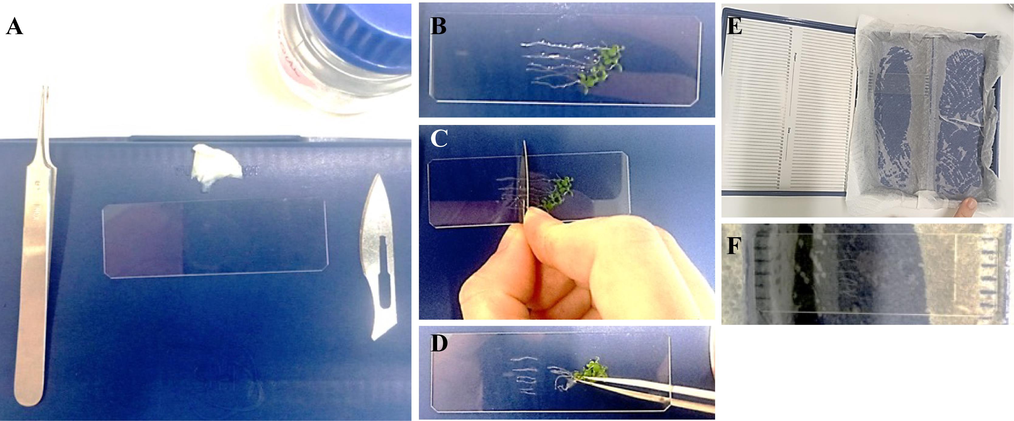
Figure 1. Slide preparation. (A) Installation of the equipment with tweezers, the SuperFrost slide, a wet Kimwipe, a razor blade, and a bottle of ultrapure water. (B) After humidification of the slide, align 5–8 seedlings. (C) Cut the roots at 3–5 mm from the tips using a razor blade. (D) Remove the rest of the seedlings. (E) Prepare the humid chamber using absorbent paper and ultrapure water. (F) After completely dry, put the slide in the humid chamber to perform the immunolabeling procedure.
A2. Cell wall digestion and membrane permeabilization
1. Create a humid chamber using a box and a wet Kimwipe paper (Figure 1E).
2. Position the slide in the humid chamber (Figure 1F).
Caution: The entire procedure needs to be done in the humid chamber to protect the sample from drying.
3. Draw a rectangle around the root tips with the hydrophobic pen.
4. Re-hydrate the sample for 5 min at 22 °C with 150 μL of MTSB 1×.
Note: The volume depends on the rectangle area, but is generally between 150 and 200 μL.
5. Incubate in cell wall digestion buffer for 30 min at 22 °C.
Caution: Driselase is a carcinogen; wear appropriate equipment and manipulate under a flow hood.
6. Wash three times for 5 min with 200 μL of MTSB 1×.
7. Incubate the sample in permeabilization buffer for 45 min at 22 °C.
8. Wash three times for 5 min with 200 μL of MTSB 1×.
A3. Immunolabeling
Note: Immunolabeling can be done using primary/secondary antibodies and/or nanobodies. If the experiment requires a primary/secondary antibody plus a nanobody, then the nanobody and the primary antibody can be mixed and incubated simultaneously.
1. Incubate the sample in blocking buffer for 1 h at 22 °C.
2. Proceed with labeling as follows:
Note: If other antibodies or nanobodies are required, please refer to the “alternative labeling strategies” notes in the Recipe section.
a. Prepare 200 μL of primary antibody solution and add 0.5 μL of GFPbooster.
b. Incubate with 200 μL of primary antibody + GFPbooster ATTO647N solution for 2 h at 37 °C.
Note: The primary antibody can be incubated overnight at 4 °C if necessary.
c. Wash four times for 5 min with 200 μL of MTSB 1×.
d. Incubate with 200 μL of secondary antibody solution for 90 min at 37 °C.
e. Wash four times for 5 min with 200 μL of MTSB 1×.
f. Incubate with 200 μL of nanobody solution for 90 min at 37 °C.
g. Wash four times for 5 min with 200 μL of MTSB 1×.
A4. Slide mounting
1. Wash for 5 min with 200 μL of ultrapure distilled water.
2. Remove the excess water and add a 15 μL drop of Mowiol.
3. Place a 22 × 22 mm 1.5 coverslip on the sample without creating air bubbles.
4. Seal with nail polish.
5. Let the mounting medium harden for 48 h at room temperature.
Note: Slides can be stored at 4 °C for several weeks.
B. Imaging
1. Turn on the microscope.
2. Start the LASX software. A window appears with three different modes; turn on the STED mode.
3. In the Configuration tab, select the laser pad: turn ON the white laser and set it to 70%, turn ON the 592 and 775 nm depletion lasers, and set them to 100%.
4. In the Configuration tab:
a. Select Objective pad: select 93× glycerol immersion objective.
b. Select the pad Align Beam: click on align beam. The alignment needs to be successful.
c. Select the Hardware pad: set the depth to 16-bit.
5. Gently clean the slide and the coverslip with ethanol to remove dust.
6. Put a drop of glycerol on the 93× glycerol objective.
7. Put a drop of glycerol on the coverslip.
8. Place the slide on the microscope stage.
9. Find the root tip and click on live to perform the focus.
Note: If finding the sample at 93× is too difficult, then change to a 20× IMM or a 20× dry objective.
10. Adjust the motorized correction ring of the objective:
Note: Precise adjustments of the motCORR can compensate for deviations in the coverslip thickness, refractive index mismatches/specimen inhomogeneities, and temperature changes to ensure restoration of optimal resolution, signal intensity, and penetration depth.
a. Select the Acquire tab.
b. Put the acquisition mode in xzy.
c. Set up the white laser to 640 nm and set the power to 1%.
d. Set up a PMT emission window to 655–675 nm.
e. Click on the AOBS configuration pad and select Reflection.
f. In the XY dialog, open the motCORR settings dialog.
g. Configure the setting by adding a value to the input field.
h. Click Live to start the acquisition and adjust the laser power appropriately without saturation.
i. Adjust the correction ring to minimize the reflection signal width corresponding to maximum intensity; see Figure 2 for optimized and non-optimized settings.
j. Once the motor collar is adjusted, restore the acquisition mode to xyz: see Figure 2 for optimized and non-optimized settings.
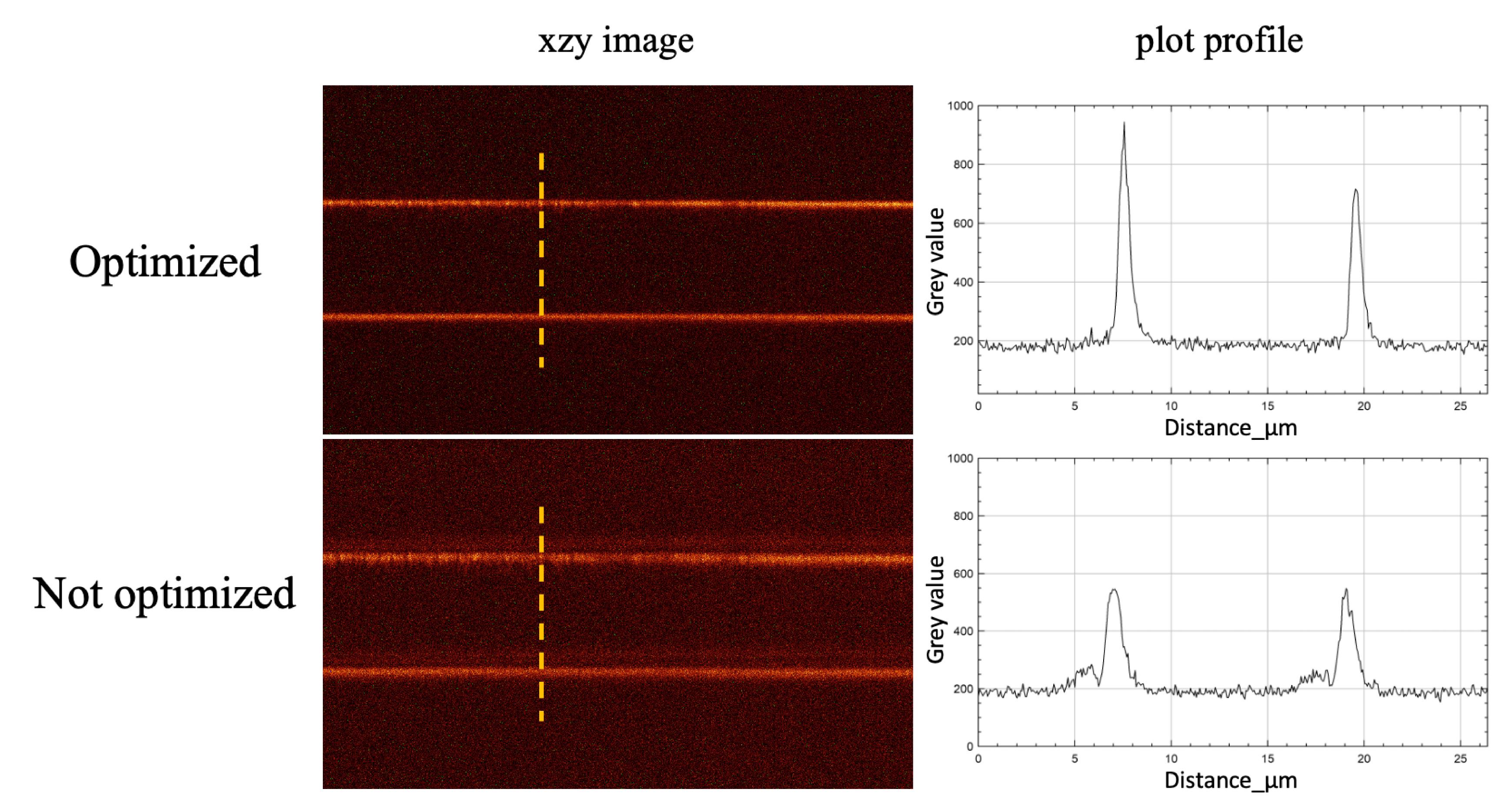
Figure 2. Objective motorized correction collar optimization. The correction collar is optimal when the signal is sharp, and the signal-to-noise ratio is improved (upper panel, plot profile along the dashed line) as compared to the non-optimized image (lower panel, plot profile along the dashed line).
B1. CONTROL: Slides with individual labeled markers
1. Acquisitions are done in sequential mode; thus, create a first sequence for the far-red channel (Table 1).
Table 1. Fluorescence excitation and emission settings of the fluorophores
| Fluorophore | Excitation wavelength (nm) | Emission window (nm) |
|---|---|---|
| Alexa Fluor 594 | 594 | 610–630 |
| Star 635P | 633 | 650–670 |
| ATTO647N | 640 | 655–675 |
2. Select a notch filtered line of the white light laser.
3. Select a hybrid detector and set up the emission window (Table 1).
4. Set the hybrid detector to 100%.
5. Click on Live and zoom in on the cell of interest.
6. Set up the laser power to reach the best dynamic range using QLut color coding of the images without saturation.
7. Pixel size needs to be 20 × 20 nm. If the entire cell cannot be captured, adjust the format of the image to obtain the required pixel size.
8. Acquire a confocal image of your region of interest (ROI); this image is required to evaluate the quality of the STED images.
9. Activate the FLIM module; the signal will be accumulated all along the acquisition, allowing the generation of a phasor plot that represents the lifetime of all the photons collected.
10. Acquire a confocal image of your ROI; this image is required to evaluate the depletion efficiency on the structure of interest (SOI) and on the photon lifetimes.
11. Activate the 775 nm depletion laser and set the power to 20%.
Note: The closer the fluorophore is to the depletion laser, the less depletion power is required.
12. Set up line repetition to 4 and acquire a STED image.
13. In the FLIM window, select the tau-STED tab and check background suppression.
Note: Background suppression allows filtering out the nonspecific signal coming from the noise, background, and reflection.
14. The selection of the “gated-STED” allows the visualization of the conventional STED image without application of the tau algorithm; see Figure 3 for a comparison between gated-STED and tau-STED.
Note: tau-strength in tau-STED microscopy refers to the gradient applied to the photon population on the phasor plot. A higher tau-strength means:
i. Stronger filtering of short-lifetime photons, which typically originate from the edges of the point spread function (PSF) (i.e., the periphery of the STED depletion doughnut).
ii. Less filtering of long-lifetime photons, which are the signature of photons emitted from the center of the doughnut, where depletion is not effective.
In essence, tau-strength modulates the selectivity of the phasor-based filter: it enhances the contrast between high-resolution signal (long lifetimes, center of the doughnut) and low-resolution or noise contributions (short lifetimes or background). By adjusting the lifetime-based filtering gradient to prioritize photons from the doughnut center, it improves resolution by suppressing unwanted photon contributions (e.g., reflections, autofluorescence, or incomplete depletion).
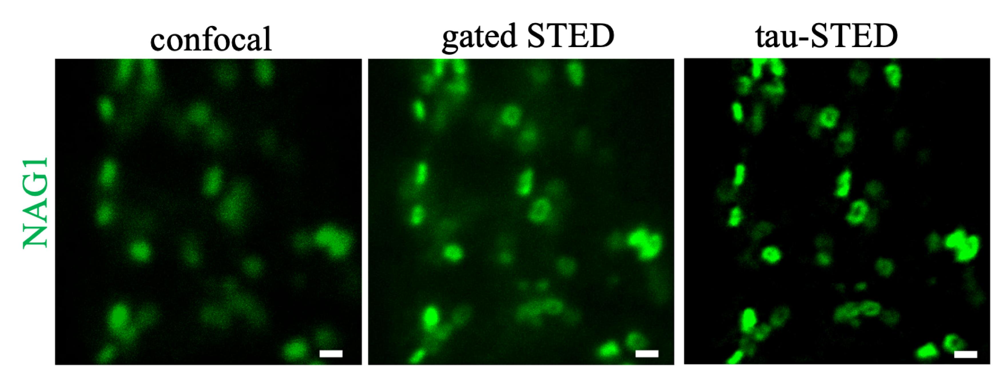
Figure 3. Comparison between confocal, gated-STED, and tau-STED images of the same cell expressing NAG1-GFP. This figure aims to show the efficiency of tau-STED as compared to the conventional gated STED (software post-processing gated-STED); in the experiments, only tau-STED images will be acquired and analyzed. NAG1-EGFP was labeled using GFPbooster ATTO647N. Scale bars, 500 nm.
15. The denoising function removes the “salt and pepper” of the images.
16. To assess the quality of the tau-STED image, two parameters are critical based on the quantity of signal per pixel. In order to evaluate the quantity of photons per pixel, right-click on the image in the FLIM window and select show data cursor.
a. The mean number of photons per pixel needs to be at least 60. Set the number of line accumulation to obtain a sufficient mean number of photons per pixel without saturation.
Note: If the optimal number of photons cannot be reached, then the tau-STED imaging cannot be successful; either the fluorescence is too dim and the immunolabeling needs to be improved, or the marker per se is too weak and not compatible with STED imaging.
b. Optimize the depletion laser power.
Note: The default tau-strength is set to 100. Acquisition parameters should be optimized to obtain high-quality images without altering this value. The tau-strength adjustments described below are solely intended for depletion parameter optimization.
i. Point the cursor to a black area of the image close to the SOI; the cursor should not show a negative value below -0.05.
ii. In the tau-STED pad, the strength of selection applied to the photon population can be modified. This tau-strength can be used to assess whether the depletion efficiency is optimal (Figure 4).
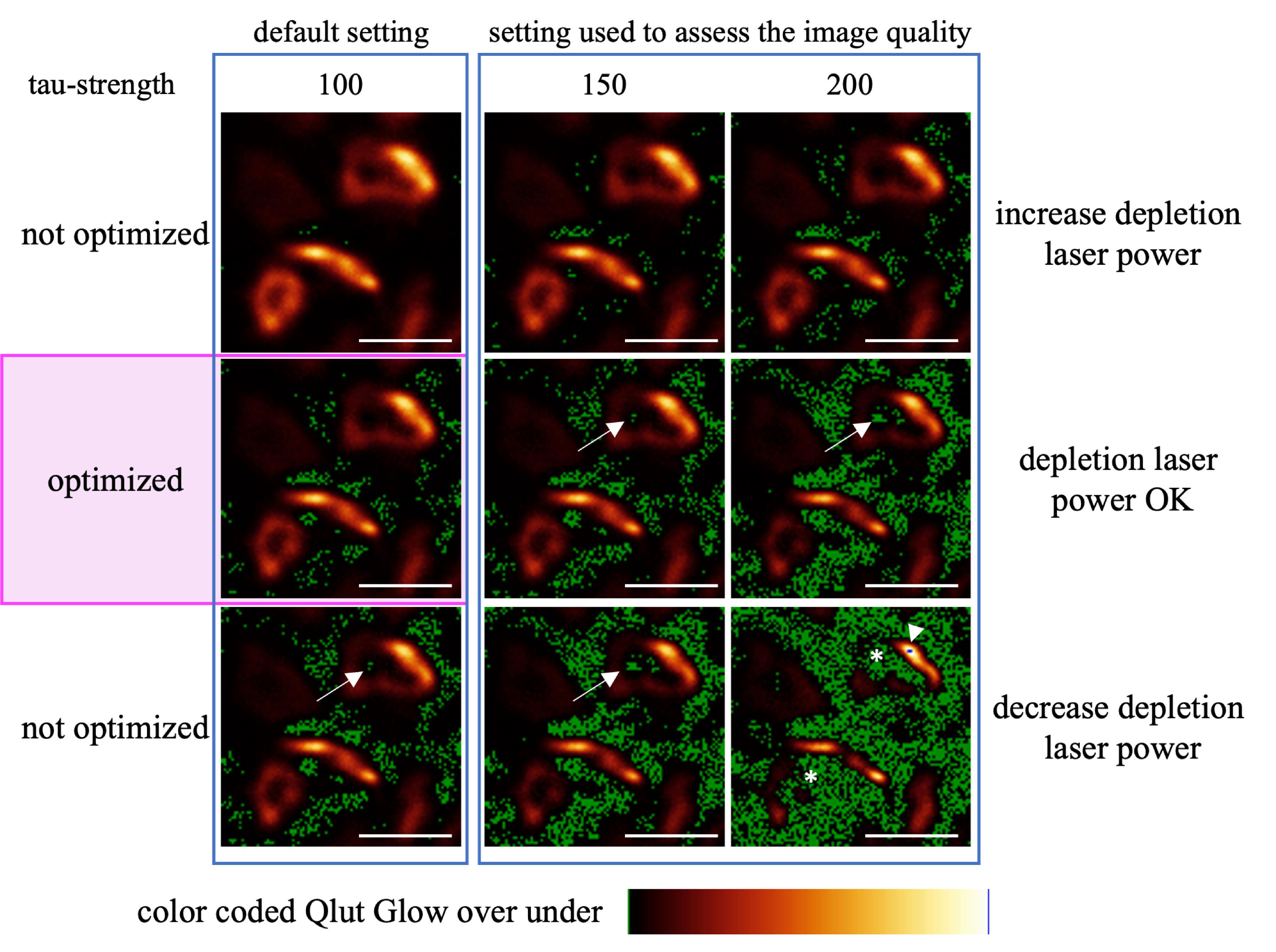
Figure 4. Depletion laser power optimization. The tau-strength refers to the selection strength applied to the photon population. By default, this value is set to 100, while the two other strength settings are solely used to assess whether the resolution of the structure is optimal. (Upper panel) No negative values can be detected in the compartments, regardless of the tau-strength applied. Thus, the depletion laser power can be slightly increased. (Middle panel) No negative values are observed at tau-strength 100, but some begin to appear inside the compartment (white arrows) as the tau-strength increases. In this case, the depletion laser power is optimal. (Lower panel) A few negative values are already visible at tau-strength 100 (white arrows), some pixels appear saturated (white arrowhead), and parts of the compartment are no longer visible (white star). Here, the depletion laser power is too strong and should be decreased. NAG1-EGFP was labeled using GFPbooster ATTO647N. Color-coded QLut Glow over under: pixels with intensity over 250 are blue and under 0 are green. Scale bars, 500 nm.
17. Set the tau-strength back to the default value (100).
18. Acquire a new tau-STED image and repeat from step B1.10 until an optimal setting is reached.
19. Create a new sequence for the AF594 and repeat steps B1.1–18 (Table 1).
20. Register the sequence.
B2. Experiment
1. Acquire a confocal image of the two channels.
2. Acquire a tau-STED image of the two channels using the previous optimized settings (Figure 5); image quality should not be affected.
Note: Sometimes, the combination of two markers and the labeling density may induce changes to the fluorophore photophysical properties. If changes are observed, repeat step B1.10–18 on both markers to adjust excitation and depletion parameters to reach an optimal quality image.
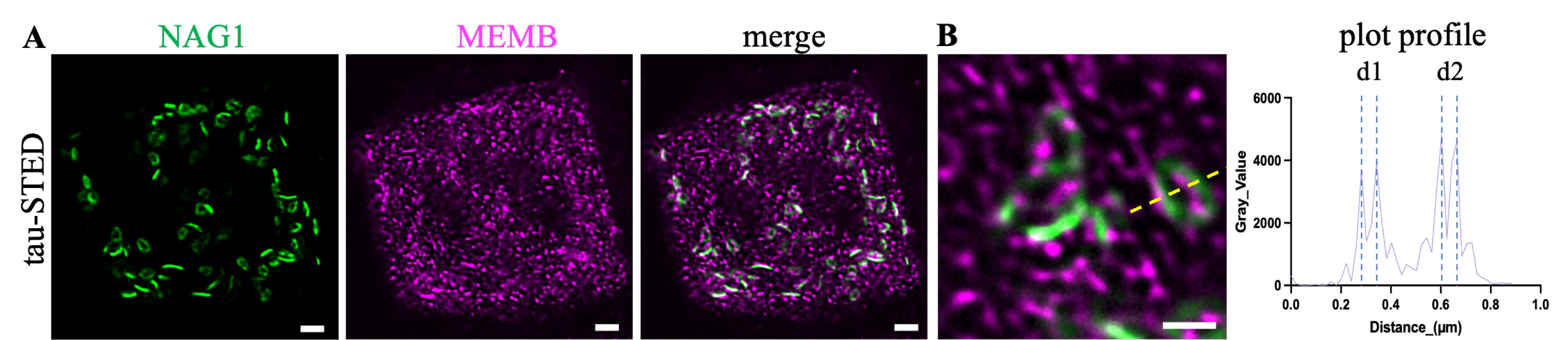
Figure 5. Golgi compartment imaged after tau-STED optimization. (A) tau-STED images of the medial-Golgi (NAG1-EGFP) and ERGIC (anti-MEMB) after optimization. (B) Magnification of the merged tau-STED image and plot profile along the dashed line. The distance between the two peaks is 61 and 63 nm for d1 and d2, respectively. Green: NAG1-EGFP labeled with GFPbooster ATTO647N; magenta: anti-MEMB labeled with anti-rabbit AF594. Scale bars, 1 μm (A) and 500 nm (B).
3. Acquire 3–5 images per root in at least three different roots.
4. Right-click on the image in the FLIM window and export the raw image.
5. Select autorange and register; each channel image will be exported in .tiff format suitable for analysis with FIJI.
Note: The experiment “.lif” needs to be conserved for the metadata, but cannot be easily opened with FIJI, as each tau-STED image will generate more than 30 different images coming from the algorithm and the photon detection. Thus, it is recommended to open the .lif in LasX software and save the .tif images in a new folder.
Data analysis
1. Open FIJI, ImageJ software.
2. Drag and drop the images (Figure 6A).
Note: The use of a color-coded LookUp Table (LUT) is recommended for a better representation of the fluorescence dynamic.
3. Duplicate the original image: Maj + D.
4. Split the channels and work on the channels one by one: Image > Color > Split Channels.
5. If necessary, the images can be filtered using Process > Filter > Gaussian blur to remove salt and pepper prior to threshold adjustment (Figure 6B).
6. Set the threshold to 50 (Figure 6C): Image > Adjust > Threshold.
Note: The threshold should be adjusted as carefully as possible to avoid losing or creating structures.
7. Make a binary image: Process > Binary > Make Binary.
8. In Set Measurements, select Shape descriptors, area, and display label: Analyse > Set measurement.
9. Run Analyze particles (Figure 6D): Analyze > Analyze particles.
a. Size (μm2): 0.05–infinity.
b. Circularity: 0.00–1.00.
c. Select: Exclude on edges and Add to manager.
d. Save all the ROIs created inside the ROI manager.
Note: The minimal object size depends on the structures that need to be detected. If the Analyze Particles detects objects that are not supposed to be detected or if it does not detect all the objects, the minimal size of detection can be adjusted.
10. The results are available in the Results window (Figure 6E).
Note: For data management, it is recommended to keep the original image and save the different treated images in a new folder.
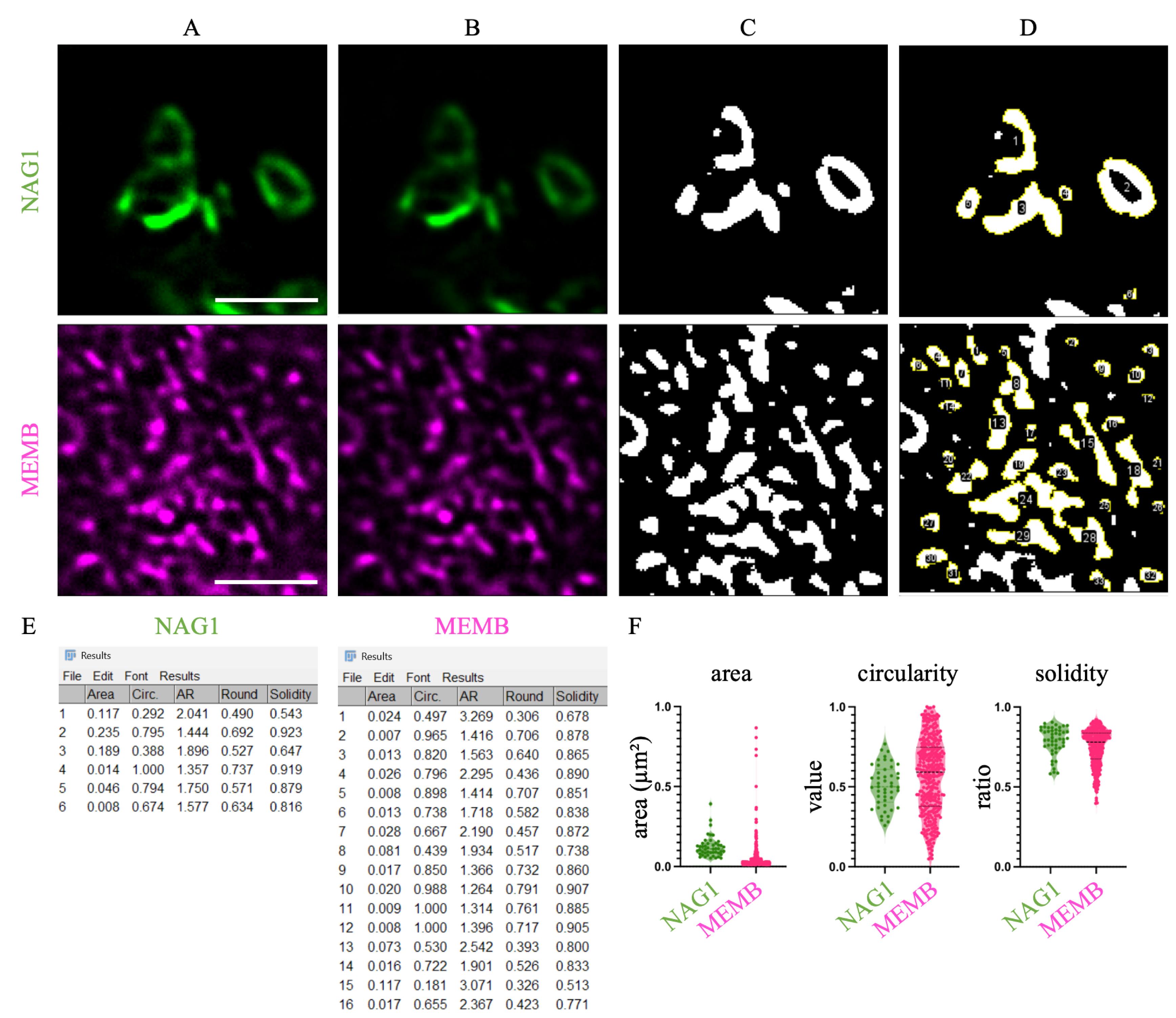
Figure 6. Morphometry analysis workflow on Tau-STED images of NAG1 (upper panel) and MEMB (lower panel). (A) Original tau-STED images. (B) Filtered images. (C) Binary image. (D) Image with the Analyze Particles drawn. (E) Results windows indicating the area, circularity (Circ.), and solidity of each object detected for NAG1 (left table) and MEMB (right table). (F) Violin plots of the area, circularity, and solidity for the two channels. Green: NAG1-EGFP labeled with GFPbooster ATTO647N; magenta: anti-MEMB labeled with anti-rabbit AF594. Scale bars, 1 μm.
Validation of protocol
This protocol has been used and validated in the following research article(s):
• Fougère et al. [8]. ER-to-Golgi trafficking through a dynamic intermediate cis-Golgi tubular network in Arabidopsis. Nature Cell Biology (Figure 5a–i, k–s; Figure 6a–d, f–i, k–s, u–ac; Extended data Figure 6c–h, j–r). https://doi.org/10.1038/s41556-025-01624-x.
General notes and troubleshooting
General notes
This protocol provides a robust and reproducible method for dual-color tau-STED super-resolution microscopy in Arabidopsis root cells in the meristematic zone. The immunolabeling procedure builds on the Nature Protocol by Boutté and Grebe [11], and the tau-STED is a technological development of Leica Microsystem’s description in Nature Methods [5]. Until recently, STED was considered inefficient in plant tissue because the depletion laser induces a background, most probably coming from very dense subcellular compounds. The tau-STED, by removing the background photons and by increasing the “weight” of the non-depleted photons, makes tau-STED really efficient in plants and opens new doors for plant cell biologists.
This protocol is optimized for Arabidopsis root tips; adapting it to other tissues may present challenges. We advise users to begin with well-characterized markers when exploring tau-STED. For applications in other plant species or tissue types, we have published a study on tomato mesocarp detailing the fixation and immunolabeling procedures, though we have not yet tested these samples with tau-STED [12]. For cleared samples, we recommend evaluating the properties of the fluorophores, ATTO647N and AF594, after ePro-ClearSee treatment [13].
Troubleshooting
| Problem | Possible cause | Solution | |
| 1 | The fluorescence signal is too low | The immunolabeling is not optimal | Double the antibodies/nanobodies concentration and/or increase the incubation time to overnight at 4 °C. |
| 2 | The fluorescence signal is heterogeneous | The marker observed may be differently expressed depending on the cell lineage | Image only the cell file allowing tau-STED imaging. |
| The immunolabeling is not optimal | Double the antibodies/nanobodies concentration and/or increase the incubation time to overnight at 4 °C. | ||
| 3 | There is bleedthrough between the channels | The labeling is too strong | Decrease the antibodies/nanobodies concentration or invert the fluorophore to position the strongest signal in the far-red channel (e.g., Star635P or ATTO647N). |
| 4 | There is a radiance effect on the image (Figure 7A) | The laser reflects on the coverslip | Shift the laser emission window until there is no more reflection. |
| 5 | The depletion induces holes in the cell (Figure 7A) | The laser reflects on the coverslip | Shift the laser emission window until there is no more reflection. |
| 6 | The depletion is poorly effective (Figure 7B) | The mounting medium is not dry | Let the Mowiol dry for at least 48 h. |
| The Mowiol is not properly prepared | Prepare a new batch of Mowiol. | ||
| 7 | There are crystals at the surface of the sample (Figure 7C) | The Mowiol pH is not correct | Prepare a new stock of Mowiol. |
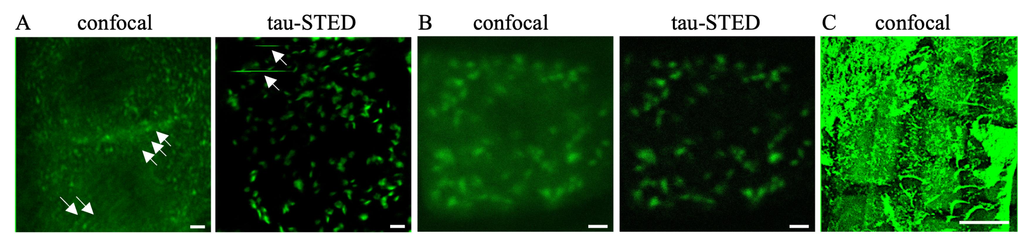
Figure 7. Troubleshooting. (A) Two different images of laser reflection on the coverslip in confocal or tau-STED images (white arrows). (B) Confocal and tau-STED images of the same cell showing a poorly effective depletion. (C) Crystals at the surface of the sample due to a wrong pH of the Mowiol. Scale bars: 1 µm (A, B) and 5 µm (C).
Acknowledgments
Imaging was performed at the Bordeaux Imaging Center (BIC), a part of the National Infrastructure France–BioImaging supported by the French National Research Agency (ANR-24-INBS-0005 FBI BIOGEN). We thank the staff of the BIC for providing support with protocol optimization and microscopy imaging. The study was supported by the grants ANR FATROOT (ANR-21-CE13-0019-02) and ANR DIVFUSE (ANR-22-CE92-0038-01). Louise Fougère was funded by a PhD MESRI fellowship from the French government and distributed through the Doctorate School in Life and Health Sciences of Bordeaux.
Contributions of each author: Conceptualization, L.F., C.P., and M.S.G.; Investigation, L.F., C.P., and M.S.G.; Writing—Original Draft, L.F., C.P., and M.S.G.; Writing—Review & Editing, L.F., C.P., Y.B., and M.S.G.; Funding acquisition, Y.B.; Supervision, Y.B. and M.S.G.
The protocol described here is based on the previous work published in Fougère et al. [8].
Competing interests
The authors declare no conflict of interest.
References
- Hell, S. W. and Wichmann, J. (1994). Breaking the diffraction resolution limit by stimulated emission: stimulated-emission-depletion fluorescence microscopy. Opt Lett. 19(11): 780. https://doi.org/10.1364/ol.19.000780
- Vicidomini, G., Bianchini, P. and Diaspro, A. (2018). STED super-resolved microscopy. Nat Methods. 15(3): 173–182. https://doi.org/10.1038/nmeth.4593
- Lanzanò, L., Coto Hernández, I., Castello, M., Gratton, E., Diaspro, A. and Vicidomini, G. (2015). Encoding and decoding spatio-temporal information for super-resolution microscopy. Nat Commun. 6(1): e1038/ncomms7701. https://doi.org/10.1038/ncomms7701
- Wang, L., Chen, B., Yan, W., Yang, Z., Peng, X., Lin, D., Weng, X., Ye, T. and Qu, J. (2018). Resolution improvement in STED super-resolution microscopy at low power using a phasor plot approach. Nanoscale. 10(34): 16252–16260. https://doi.org/10.1039/c8nr03584a
- Alvarez, L., Schwartz, U., Friedrich, L., Foelling, J., Hecht, F. and Roberti, J. (2021). TauSTED: pushing STED beyond its limits with lifetime. Nat Methods. 12: 3463.
- Becker, W. (2021). The bh TCSPC handbook. Becker & Hickl GmbH.
- Becker, W., Shcheslavskiy, V. and Bergmann, A. FLIM at a Time-Channel Width of 300 Femtoseconds. Education Brochure [date unknown].
- Fougère, L., Grison, M., Laquel, P., Montrazi, M., Cordelières, F., Fernández-Monreal, M., Poujol, C., Uemura, T., Nakano, A., Ito, Y., et al. (2025). ER-to-Golgi trafficking through a dynamic intermediate cis-Golgi tubular network in Arabidopsis. Nat Cell Biol. 27(3): 424–437. https://doi.org/10.1038/s41556-025-01624-x
- Geldner, N., Dénervaud-Tendon, V., Hyman, D. L., Mayer, U., Stierhof, Y. D. and Chory, J. (2009). Rapid, combinatorial analysis of membrane compartments in intact plants with a multicolor marker set. Plant J. 59(1): 169–178. https://doi.org/10.1111/j.1365-313x.2009.03851.x
- Marais, C., Wattelet-Boyer, V., Bouyssou, G., Hocquellet, A., Dupuy, J. W., Batailler, B., Brocard, L., Boutté, Y., Maneta-Peyret, L., Moreau, P., et al. (2015). The Qb-SNARE Memb11 interacts specifically with Arf1 in the Golgi apparatus of Arabidopsis thaliana. J Exp Bot. 66(21): 6665–6678. https://doi.org/10.1093/jxb/erv373
- Boutté, Y. and Grebe, M. (2013). Immunocytochemical Fluorescent In Situ Visualization of Proteins In Arabidopsis. Methods Mol Biol. 1062: 453–472. https://doi.org/10.1007/978-1-62703-580-4_24
- Beauchet, A., Bollier, N., Grison, M., Rofidal, V., Gévaudant, F., Bayer, E., Gonzalez, N. and Chevalier, C. (2023). The FW2.2/CNR protein regulates cell-to-cell communication in tomato by modulating callose deposition at plasmodesmata. bioRxiv.: e559775. https://doi.org/10.1101/2023.09.27.559775
- Nagaki, K., Yamaji, N. and Murata, M. (2017). ePro-ClearSee: a simple immunohistochemical method that does not require sectioning of plant samples. Sci Rep. 7(1): e1038/srep42203. https://doi.org/10.1038/srep42203
Article Information
Publication history
Received: Apr 23, 2026
Accepted: Jun 21, 2026
Available online: Jul 9, 2026
Published: Aug 5, 2026
Copyright
© 2026 The Author(s); This is an open access article under the CC BY-NC license (https://creativecommons.org/licenses/by-nc/4.0/).
How to cite
Fougère, L., Poujol, C., Boutté, Y. and Grison, M. (2026). Dual Color tau-STED Super Resolution Microscopy in Arabidopsis Root Tip. Bio-protocol 16(15): e5774. DOI: 10.21769/BioProtoc.5774.

 Download Citation in RIS Format
Category
Plant Science > Plant cell biology > Cell imaging
Plant Science > Plant cell biology > Cell structure
Do you have any questions about this protocol?
Post your question to gather feedback from the community. We will also invite the authors of this article to respond.
 Post a Question


