


- Protocols

- Articles and Issues
- For Authors
- About
- Become a Reviewer


Computational Quantification of Mouse Retinal Vasculature Using ImageJ

Published: Vol 16, Iss 11, Jun 5, 2026 DOI: 10.21769/BioProtoc.5705 Views: 506
Reviewed by: Nona FarbehiAbhishek VatsMatt Govendir
 PDF
PDF  Ask a question
Original research article
The authors used this protocol in:

Feb 2026
Advertisement



Protocol Collections
Comprehensive collections of detailed, peer-reviewed protocols focusing on specific topics




Abstract
Postnatal mouse retinal vascular development is a widely used model for studying retinal vascular diseases and evaluating candidate therapies. This is particularly relevant for inherited disorders such as familial exudative vitreoretinopathy (FEVR), in which impaired vascular growth and organization are central to disease pathogenesis. Numerous approaches have been used to assess retinal vasculature in mouse flat mounts, ranging from qualitative descriptions to limited quantitative measurements of vascular growth. However, phenotypic variability across genetic models, including different models of FEVR, complicates comparisons and underscores the need for standardized, comprehensive multi-parameter analyses that are suitable for rapid and cost-effective screening studies. We describe a standardized morphometric protocol using ImageJ software to quantitatively analyze mouse retinal vasculature in a reproducible manner. The protocol begins with measurement of areas of vascular disorganization (meshes) as well as total vascular and retinal area. Two defined regions in the peripheral and midperipheral retina are then selected to quantify cell clusters, followed by image processing, binarization, and skeletonization. From these processed images, vascular density, branch number, branch length and thickness, junction number, triple points, and box-counting fractal dimension and lacunarity are quantified. Overall, this protocol provides a rapid, cost-effective, and standardized framework for quantifying retinal vascular phenotypes across diverse mouse models. By capturing multiple structural features and accommodating phenotypic variability, it is well-suited for comparative studies and therapeutic screening in retinal vascular disease.
Key features
• Computational method for mouse retina vessel image analysis for multi-parameter vascular quantification for user-selected regions of interest.
• Free open-source ImageJ-based workflow combining disorganization mapping, skeletonization, and fractal analysis for reproducible vascular network characterization.
• Optimized for rapid, cost-effective screening of structural vascular outcomes across developmental stages, disease states, and therapeutic interventions.
Keywords: Retina Vessels
Mice
Screening tool
Disease models
Candidate treatments
Image analysis
ImageJ
FIJI
Fractal analysis
Image processing
Morphometry
Vessels
Mice
Screening tool
Disease models
Candidate treatments
Image analysis
ImageJ
FIJI
Fractal analysis
Image processing
Morphometry
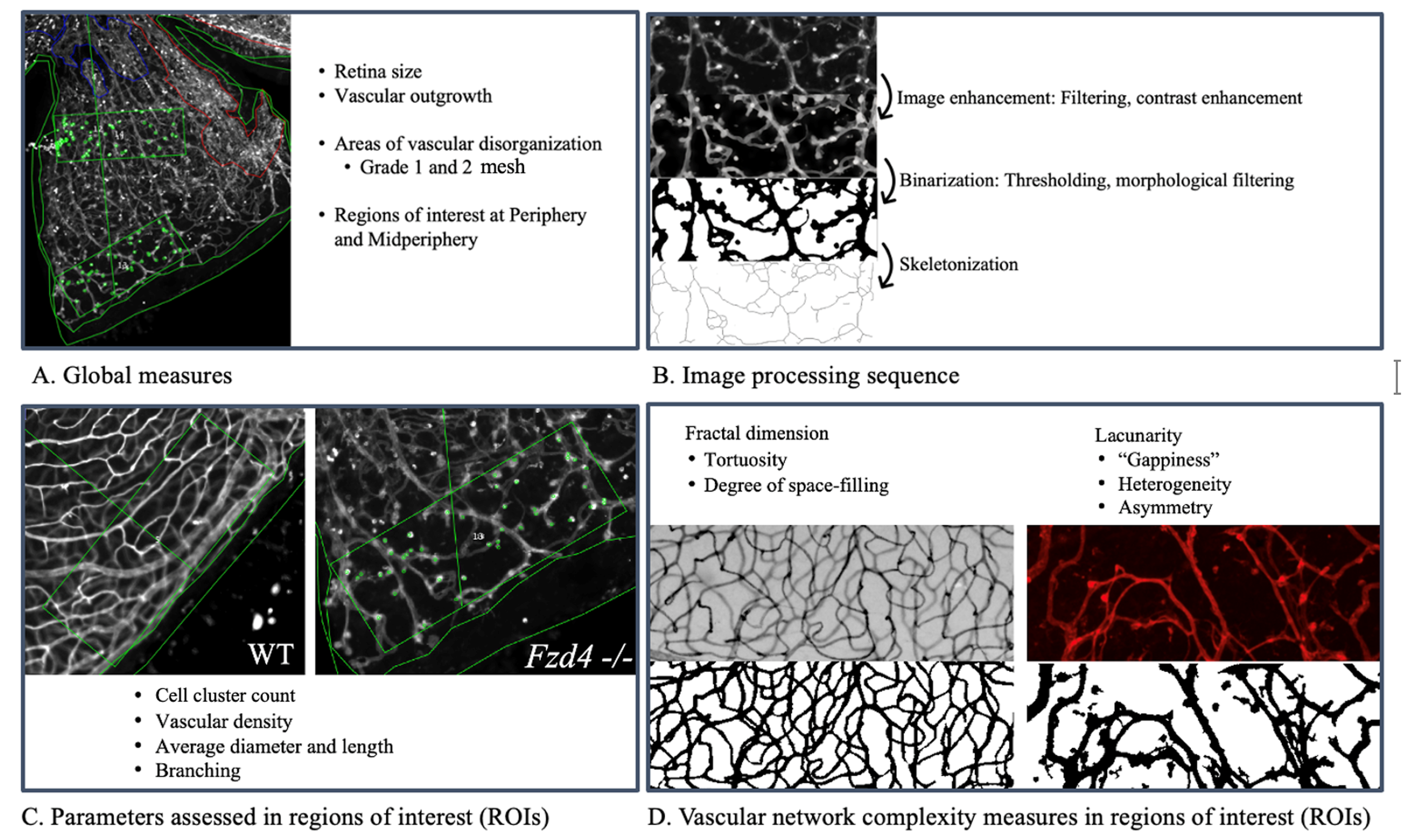
Graphical overview
Background
Development and maintenance of the retinal vasculature is essential for proper ocular function and vision. Disease states where retinal vascularization is abnormal are common causes of blindness [1–3] and include diabetic retinopathy [4–7], retinopathy of prematurity (ROP) [8–12], and inherited retinal vascular diseases exemplified by familial exudative vitreoretinopathy (FEVR) [9,13–29]. In humans, the retinal vasculature is initiated by vascular precursors that lay down the primary vessels that project radially from the optic disc to the retinal periphery by term gestation to form the superficial vascular plexus. From this plexus, starting around 25–26 weeks of gestation, secondary vessels penetrate the retina to form two networks, the deep capillary plexus, on either side of the inner nuclear layer [27–35].
In rodents, as in humans, a primary vascular bed first extends from the optic nerve to the peripheral retina in a single plane along the superficial retina, and the superficial plexus then sends sprouts vertically into the deeper layers of the retina that will form two intraretinal networks. Unlike humans, who exhibit fully formed retinal vessels by term birth, the primary vascular plexus in rodents develops in the first postnatal week, and the formation of the deeper layers is completed by postnatal day 14 (P14). Rodent models offer a unique opportunity to study the evolution of developmental retinal vascular disorders [29,34,36] and, as such, are widely used to study mechanisms of human retinal disease. To do so, retinal vasculature is often determined by flat mounts of retinas followed by staining, visualization, and analysis. However, there is no standard approach that can quantify relevant parameters and capture the phenotypic diversity observed in the various genetic and environmental mouse models, comparing them and assessing responses to candidate treatments. An extensive number of parameters can be individually quantified (Tables 1 and 2). We devised and tested a computational protocol for determining clinically relevant retinal vascular properties ranging from size to network complexity.
Other computational tools have been published in the past, such as Angiogenesis Analyzer, REAVER, Vessel Analysis, AngioQuant, RAVE, SIVA, and AngioTool, among others [37–43]. However, they do not have a wealth of scientific literature regarding their application, they are inflexible regarding which parameters are quantified and how, they are not customizable, they do not have an active developer community, most are not open source, which prevents full transparency regarding the underlying algorithms, they present financial barriers, and they are not available on multiple operating systems. Our protocol thus responds to all of these limitations by using ImageJ, a free and fully open-source software with an active community, vast customizability, compatibility across iOS, Windows, and Linux operating systems, and extensive use in the literature [44].
Global vascular development of the mouse retina depends on the postnatal age and body weight and is measured as percent vascularized area (PVA) of the total retinal area and vessel density (VD). VD is affected by the number, length, and diameter of the vessels. Therefore, we include average branch length (BL), average branch thickness (BT), number of branches (BN), number of junctions (JN, a point where a branch divides), and triple points (TP, junctions where there are two branches emerging from one) in regions of interest (ROIs) (Table 1). Together, these parameters can clarify whether a large VD consists of many small, interconnected capillaries or fewer but larger vessels.
Table 1. Parameters and techniques used to quantify retinal vascular networks and their relevant regions of interest (ROIs)
| Parameter | Description | Reference |
|---|---|---|
| Retinal area | Total area of the whole retina | N/A |
| Percent vascularized area | Proportion of total retinal area with vessels | N/A |
| Vascular outgrowth | Distance from optic nerve to vascular front | [36] |
| Vessel density | Area of the vessels divided by the total area of the ROI | [36,38,45] |
| Histogram integrated density | The product of the length of the fibers and the average radius | [46,47] |
| Vascular length | Total length of skeletonized vessels | [36, 38, 45–48] |
| Average branch length | Average length of all the branches in the network | [48–50] |
| Branch length density | Average branch length per area of ROI | N/A |
| Vessel length density | Total vessel length per area of ROI | [38,45–47] |
| Characteristic length | Total length of all centerlines (skeleton) divided by the number of intersections | [45–47] |
| Average vessel diameter | Average vessel diameter/thickness | [45–47] |
| Vessel diameter density | Average vessel diameter per area of ROI | N/A |
| Diameter histogram | Histogram of measured diameters with mean, mode, median, standard deviation, skewness, and kurtosis | [46,47] |
| Vessel Perimeter Index | Ratio between vessel perimeter and total area | [49–51] |
| Branchpoint density | Number of branching points in the skeletonized network per area | [36,38,45] |
| Branching angle | The first angle subtended between two daughter vessels at each branch point | [50–52] |
| Branching coefficient | Coefficient relating the diameter of the parent branch and the two daughter branches according to an equation | [51–53] |
| Vessel segment partitioning | Number of segments divided by total vessel segment lengths | [52–54] |
| Nearest neighbor distance | Average minimum distance and variability in distribution between the vessels in the region | [36,38,45] |
| Tortuosity | Measure of the degree of twisting and turning in the path of the vessel | [51–53] |
| Vessel Complexity Index | Index relating vessel perimeter to area | [51–53] |
Parameters such as VD, BL, BT, BN, JN, and TP rely on the assumption that defined vessels are present in a ROI, but this is not always the case. Retinas from a genetic mouse model of the childhood blinding disorder FEVR, the Fzd4-/- mouse model, may manifest large areas of vascular disorganization—termed meshes—with no defined vascular network. To capture these characteristics, each of these areas is outlined and measured, and its ratio to the total vascularized area is reported. We define meshes with a significant lack of defined vasculature as Grade 1 mesh, and areas with an almost complete lack of structure as Grade 2 mesh.
Table 2. Examples of fractal analysis methods
| Name | Reference |
|---|---|
| Box-counting fractal dimension (DB) | [53–55] |
| Information dimension | [53–56] |
| Correlation dimension | [53–56] |
| Local connected fractal dimension | [56–58] |
| Differential box-counting method | [59–72] |
| Extended box-counting method | [61–63] |
| Isarithm method | [62–64] |
| Blanket method | [64–66] |
| Triangular prism method | [65–67] |
| Hausdorff fractal dimension | [67–69] |
| Modified Hausdorff fractal dimension | [67–69] |
| Fourier fractal dimension | [68–71] |
The term complexity can relate to branching, vessel overlap, tortuosity, density, symmetry, space-filling, and the heterogeneity of any of these factors. Quantifying this complexity in our vessel networks can be addressed by applying fractal geometry (Table 2). In combination with the other quantified structural characteristics of this vessel network (e.g., length, thickness, and number), we can glean information on both the development of vessels at the local level and how that impacts the network’s global complexity and vice versa. Each approach complements the other, as they capture information from different perspectives. Fractal analysis has been used to investigate retinal vascular development in many circumstances. The box-counting fractal dimension (DB) method is the most widely utilized to analyze retinal vasculature complexity [53,60,68], thus being selected for our protocol. Box-counting fractal dimension quantifies how complex and space-filling a branching pattern is by counting how many grid boxes contain vessel segments as the box size decreases. In the context of the retinal vasculature, this measure reflects the geometric complexity and curvature of the vessel network.
Although DB is a powerful tool, it can be nonspecific, as different patterns with similar DB can remain qualitatively very different [71]. To mitigate this, lacunarity used in conjunction with fractal dimension characterizes the heterogeneity and symmetry of gaps surrounding an object and together form a more specific impression of the vascular network [71]. Lacunarity measures how evenly or unevenly a pattern fills space, capturing the size and variability of gaps within a structure. Low lacunarity indicates a uniform, tightly packed network with consistent spacing between elements, whereas high lacunarity reflects larger, more irregular gaps and a less cohesive pattern.
In this publication, we report the development of a standardized computational approach that captures and measures structural and pathological features in a mouse retina flat mount in a rapid and reproducible fashion in ImageJ tables, using the software and plugins in Table 3. More specifically, it quantifies the total retina size (μm2), the percent vascularized area (%), and the proportion of area of significant vascular disorganization (meshes) that have no definable network structure (%). Then, in chosen regions of interest at the periphery and midperiphery, we calculate VD (ratio), BL (μm), BT (μm), BN, JN, TP, number of cell clusters (CCs, microaneurysm-like structures), DB (unitless), and lacunarity (Λ unitless).
Equipment
1. Laptop or desktop computer with the required software installed. We used a MacBook Pro (2.4 GHz Quad-Core Intel Core i5/ 8 GB 2133 MHz LPDDR3/macOS 15.7.4 24G517).
Minimum requirements to download the latest versions of FIJI are:
a. Windows 10 or later, x86–64 or arm64
b. macOS 11 “Big Sur” or later, Apple Silicon or Intel
c. Ubuntu 22.04 LTS or later, x86-64 or arm64
d. Any other system with a Java 21 runtime, except plugins using native libraries (e.g., 3D Viewer)
Software and datasets
Table 3. Software and plugins used in the FIJI retinal vasculature analysis protocol
Procedure
A. Set the scale to convert pixels to μm
1. Analyze > Set Scale…
2. Use the line tool to draw over the scale bar.
3. Put in the known distance from the scale on your image and the units of measurement.
B. Set your measurements
1. Analyze > Set Measurements…
2. Select Area, Display label, Area fraction, and Add to overlay.
C. Outline the total retinal area
1. Select the polygon selection tool.
2. Outline the outer borders of the retina (Figure 1).
3. Add the overlay (Image > Overlay > Add Selection) to the ROI manager (Image > Overlay > To ROI manager).
4. Measure the outline (Analyze > Measure) and record the value.
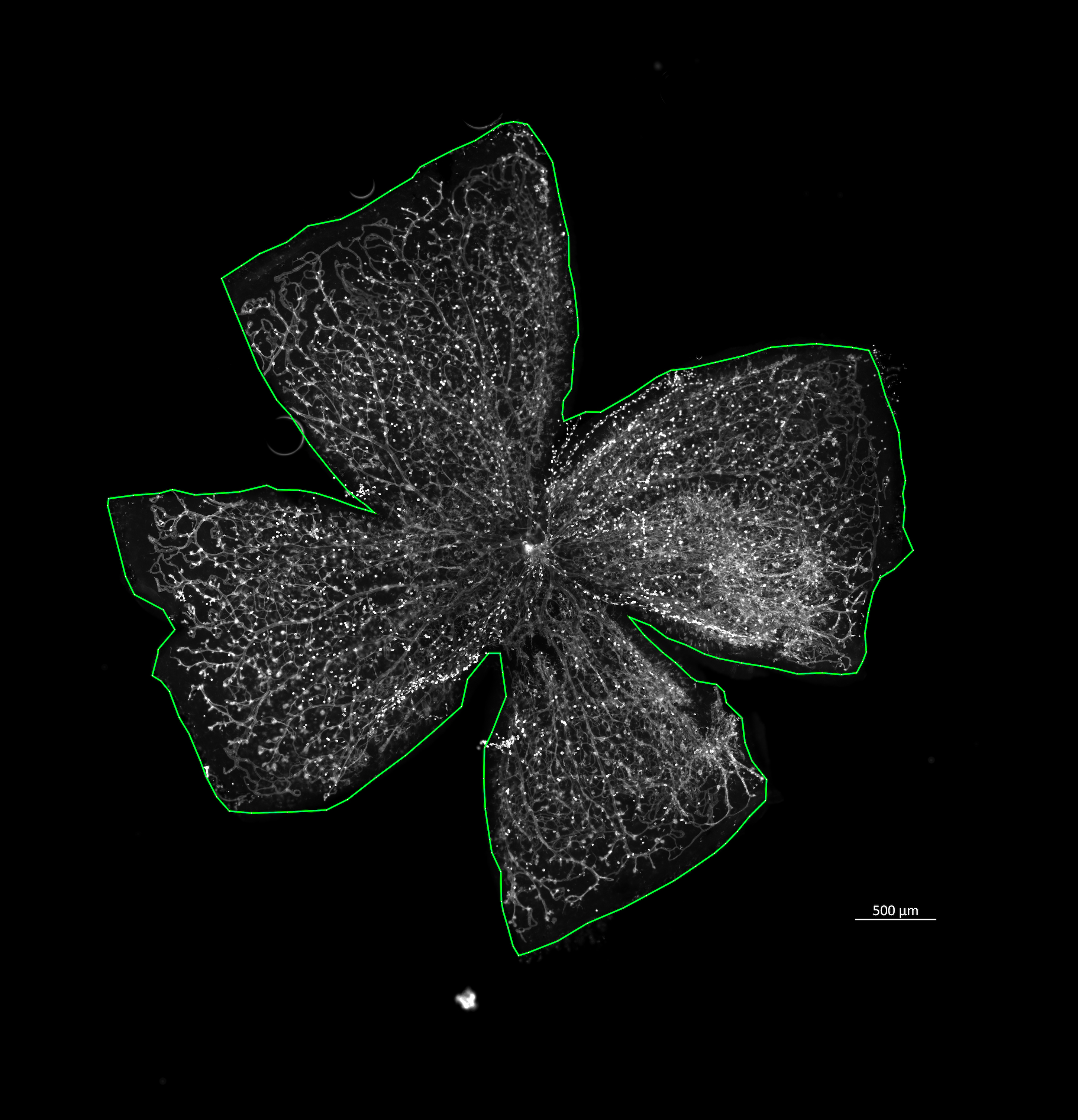
Figure 1. Whole retina flat mount image of the FZD4 mouse model with the outer border of the retina outlined. Scale bar, 500 μm.
D. Total retinal vascularized area
1. Select the polygon selection tool.
2. Outline the vascularized area of the retina up to the periphery (Figure 2).
3. Add as an overlay (Image > Overlay > Add Selection) to the ROI manager (Image > Overlay > To ROI manager).
4. Ensure that you have the vasculature outline selected when you are measuring. Measure the outline (Analyze > Measure) and record the value.
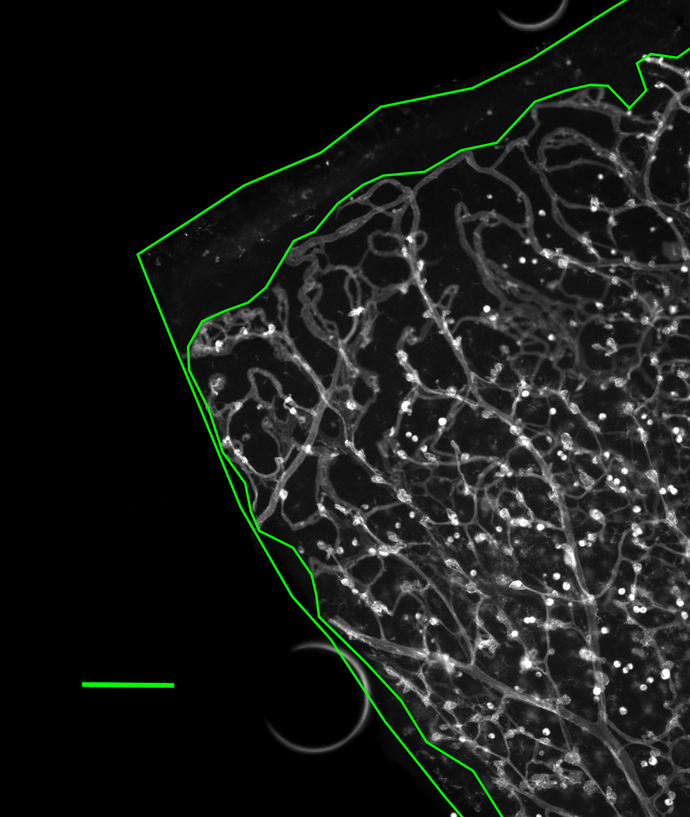
Figure 2. Enlarged corner of the whole retina image, highlighting the outer border of the retina and the peripheral border of the vascularized area. Scale bar, 200 μm.
E. Saving representative ROIs from the periphery and midperiphery
1. Choose a quadrant of interest.
2. Use the Rotated Rectangle tool to draw a 300 × 800 μm (depth × width) rectangle at the periphery of the retina following the angle of vessels (Figure 3). Avoid analyzing areas that are not representative of the overall structure of the retinal vasculature.
3. Add the ROI as an overlay to the ROI manager.
4. Draw a second 300 × 800 μm rectangle overlay at the mid-periphery of the retina in the same quadrant and add it to the ROI manager (Figure 3).
Notes: The line tool can be used to precisely locate the midway point from the center and periphery, which is what the mid-periphery ROI should cover. This is done by drawing a straight line from the center to the periphery, adding it as an overlay, and noting where the overlay numerical label marker appears, as this is the exact midpoint of that straight line.
5. Prioritize getting a quantifiable representative area, i.e., the mesh may preclude measurements in a specific region, hence the need to capture the mesh separately.
6. Repeat steps E2–5 for all quadrants of interest.
7. Duplicate each overlay from the ROI manager in sequential order to produce individual images of the selected peripheral and mid-peripheral regions in each quadrant of the retina.
8. Save images for processing.
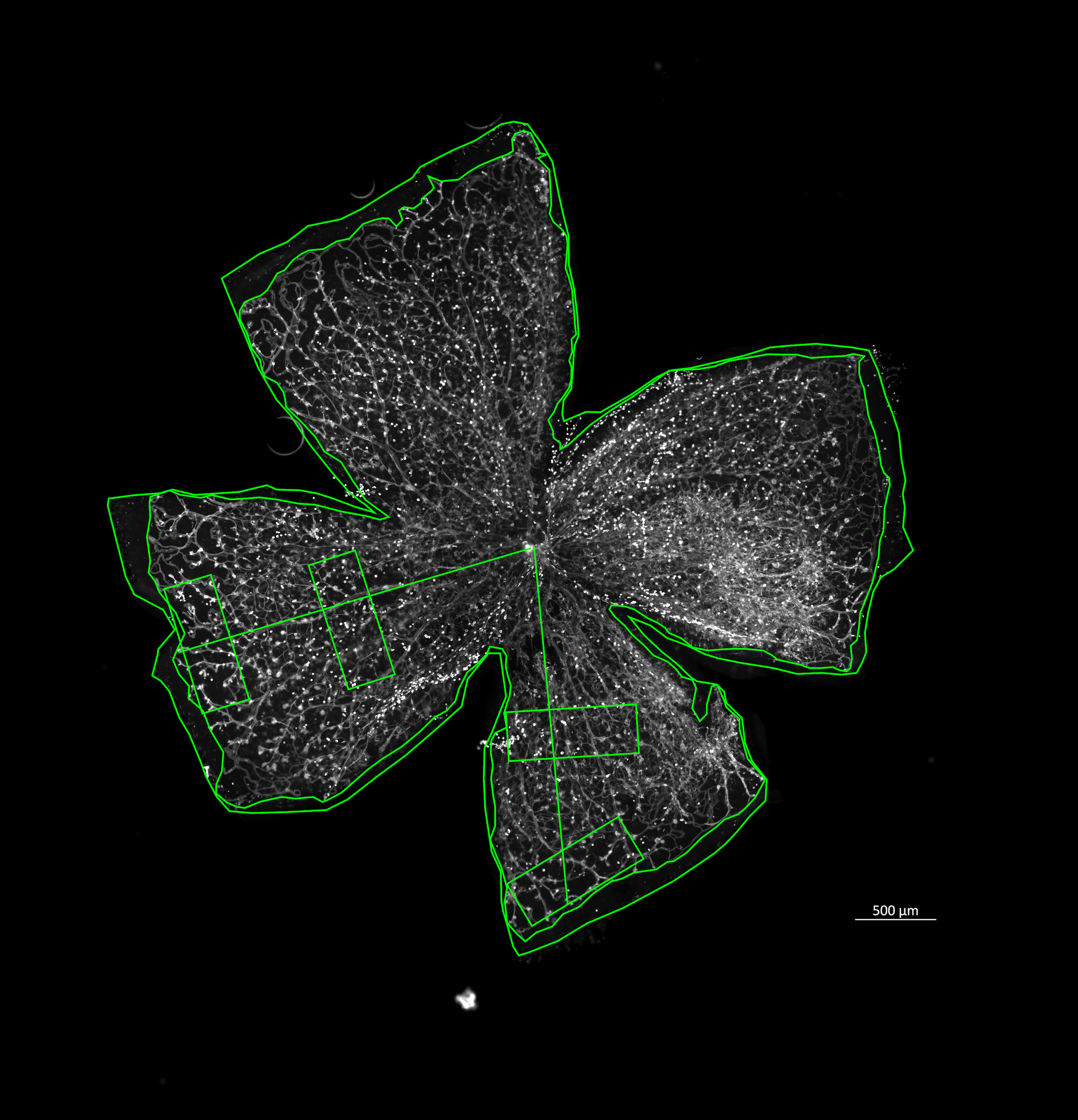
Figure 3. Whole retina flat mount image of the FZD4 mouse model with representative 300 × 800 μm regions of interest (ROIs) at the periphery and mid-periphery selected in the right and left lower quadrants of the retina, which do not contain meshes. The outer border of the retina and the vascularized area are also outlined. Scale bar, 500 μm.
F. Processing ROI images
1. Open the previously saved ROI image and duplicate it.
2. Convert the image to grayscale 8-bit if the image is in color (Image > Type > 8-bit).
3. Enhance contrast to better outline the vessels using the Enhance Local Contrast feature [Process > Enhance Local Contrast (CLAHE)] (Figure 4).
Notes:
1. This can enhance noise.
2. Blocksize is the area that is equalized.
3. Histogram bins are the number of bins used in the histogram; use the maximum number of pixels in the block up to the number of grayscale values (256 for an 8-bit image).
4. The maximum slope is the amount of contrast enhancing. Slope = 1 is the original image.
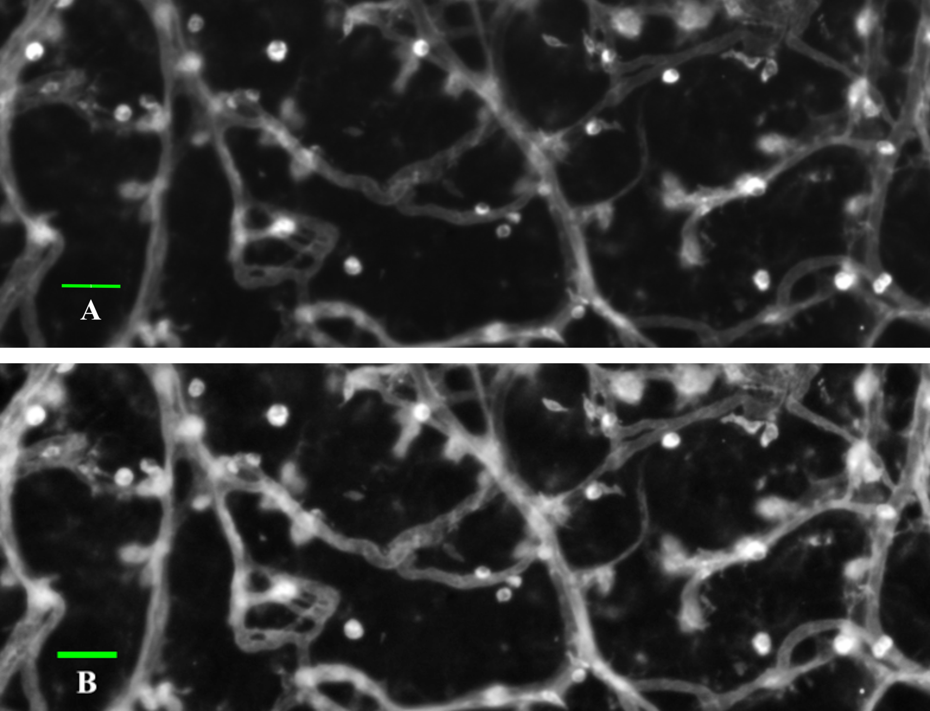
Figure 4. Representative images before (A) and after (B) contrast-limited adaptive histogram equalization (CLAHE) filtering. Scale bar, 50 µm.
4. Filter any Gaussian background noise using the non-local means denoising plugin (Plugins >Non-local means denoising) (Figure 5).
Notes:
1. This can eliminate details such as small vessels.
2. Sigma is the range or variation in noise. In practice, it is similar to the degree of averaging of the signal by the plugin.
3. Smoothing factor is the level of smoothing. Typically, keep it at 1.
4. Auto-estimate when you can, but do it manually if the level of filtering is too high or low.
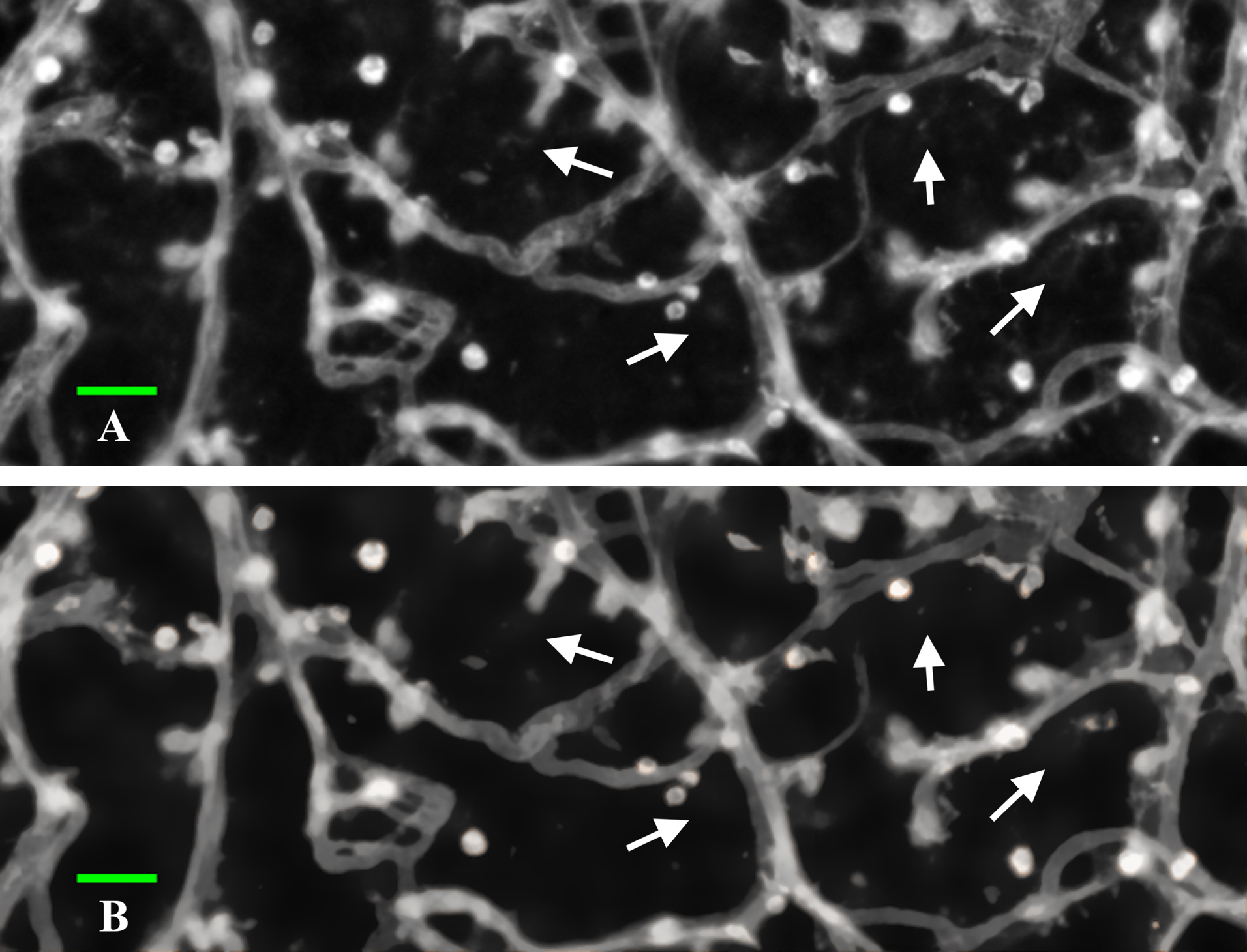
Figure 5. Representative before (A) and after (B) images after using non-local means (NLM) filtering. White arrows point to general areas where NLM successfully reduced noisy, heterogeneous sections of the image. Scale bar, 50 µm.
5. Use the Unsharp Mask filter (Process > Filters > Unsharp Mask) to enhance the edges of the vessels. This helps maintain the distinction between vessels and the details of the structure (Figure 6).
Notes:
1. This can enhance noise and worsen the heterogeneous staining of vessels, which can create artifacts when binarizing.
2. The radius is the standard deviation of the Gaussian blur that is subtracted to enhance edges.
3. Mask weight is the strength of filtering, where 1 represents infinite weight. Preview the image to optimize the parameters before finalizing.
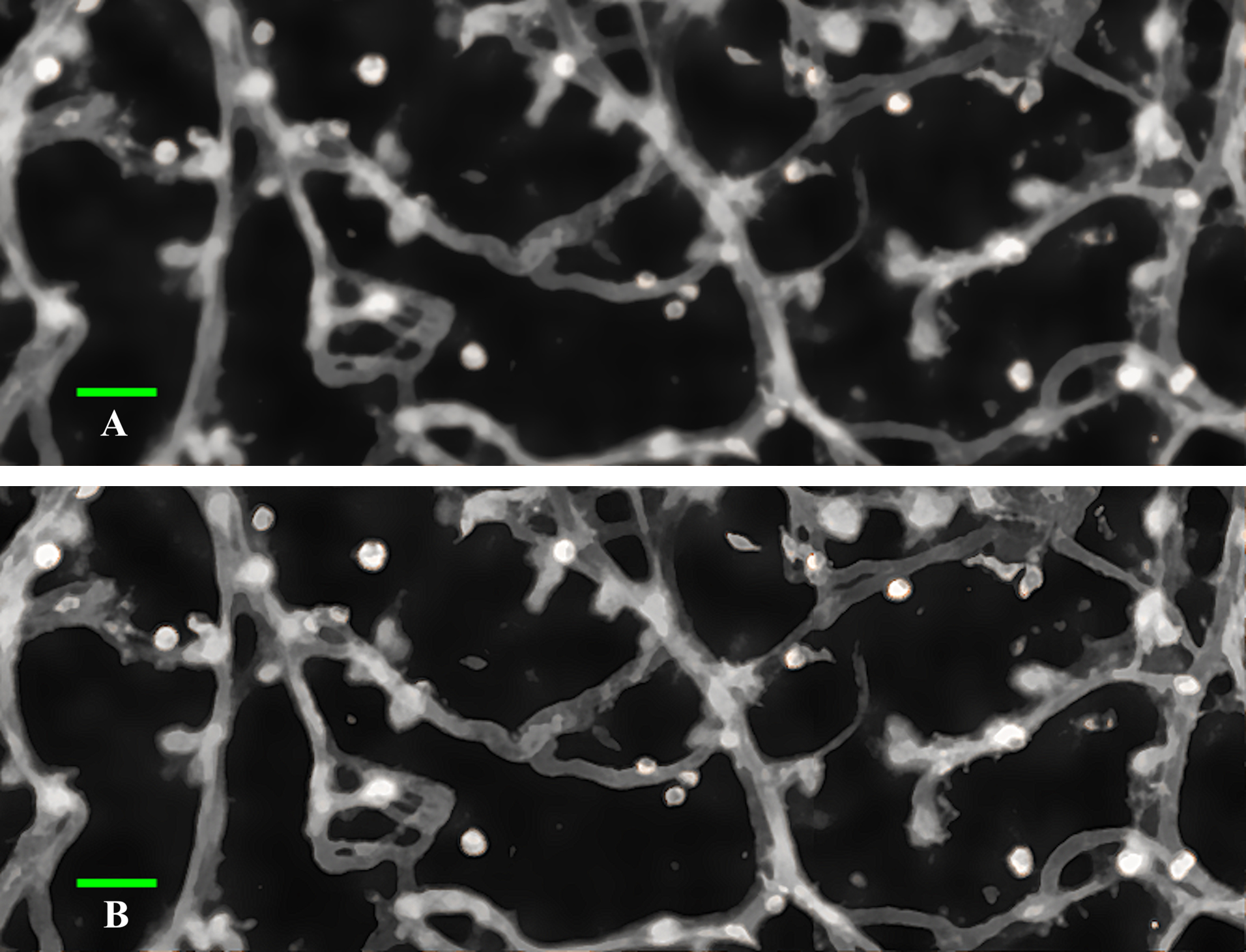
Figure 6. Representative before (A) and after (B) images after using Unsharp Mask filtering. Scale bar, 50 µm.
6. Use the median filter (Process > Filters > Median) to remove salt-and-pepper noise, i.e., high and low intensity specs in the background (Figure 7).
Notes:
1. This should preserve edges better than Gaussian, mean, or other basic local filters, but it will do some smoothing.
2. Radius is the radius of the pixels compared to set the median; the higher value, the more smoothing. Optimize by using previewing.
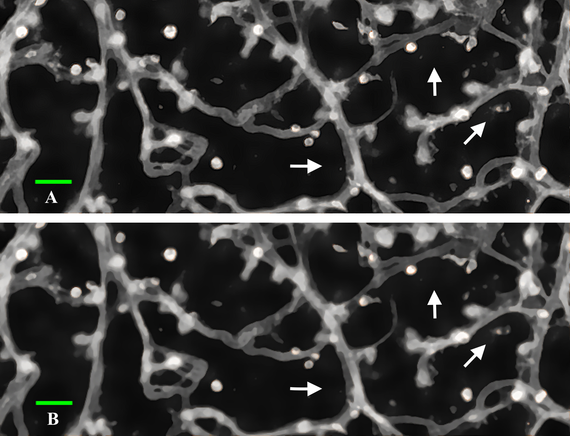
Figure 7. Representative before (A) and after (B) images after using Median filtering. White arrows indicate areas where high-intensity noise around edges was smoothed. Scale bar, 50 µm.
7. Use the Subtract function (Process > Math > Subtract) to reduce the values of all the pixels in the image by a set amount chosen by you. This can be used as the last attempt in removing a loud patch of noise that other filtering functions could not delete.
Note: This is a brute-force way to remove any remaining background noise. Subtract by the value of the pixels in the darkest part of the background or the parts you want to eliminate.
8. Binarize the image by first setting the threshold for LUT (Image > Adjust > Threshold). Adjust the threshold so that the black and white image represents the original.
9. Convert the new image to a binary image (Process > Binary > Convert to Mask) (Figure 8).
Note: Convert the image pixel values to 255 (if 8-bit) for foreground and 0 for background.
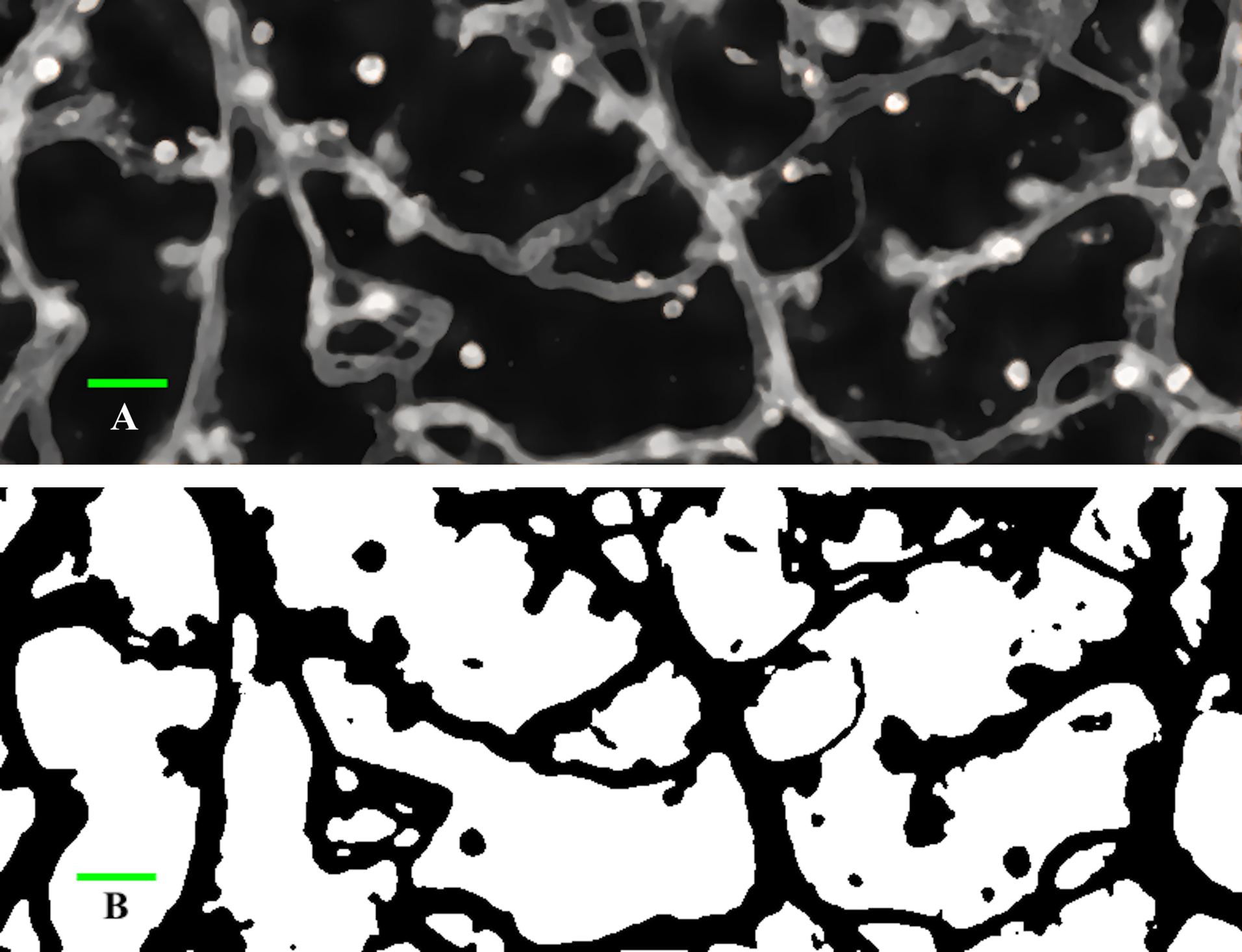
Figure 8. Representative image of a region of interest (ROI) before (A) and after (B) it has been converted to a binary image. Scale bar, 50 µm.
10. Analyze particles (Analyze > Analyze Particles…> size=100-Infinity, Show = Masks) to filter out particles with an area less than 100 μm2 (Figure 9). This size was chosen to avoid filtering out real and large structures in the image. The remaining unconnected CCs do not end up having a significant impact on the results.
a. Outline all structures and proceed with whatever operation you have set, such as counting, measuring, or removing.
b. Size sets the range of area you intend to consider.
c. Show = Masks tells the program to show the structures that fit within your range, effectively filtering out everything below or above it. In this case, as the upper bound is “infinity,” it filters any object less than 100 μm2.
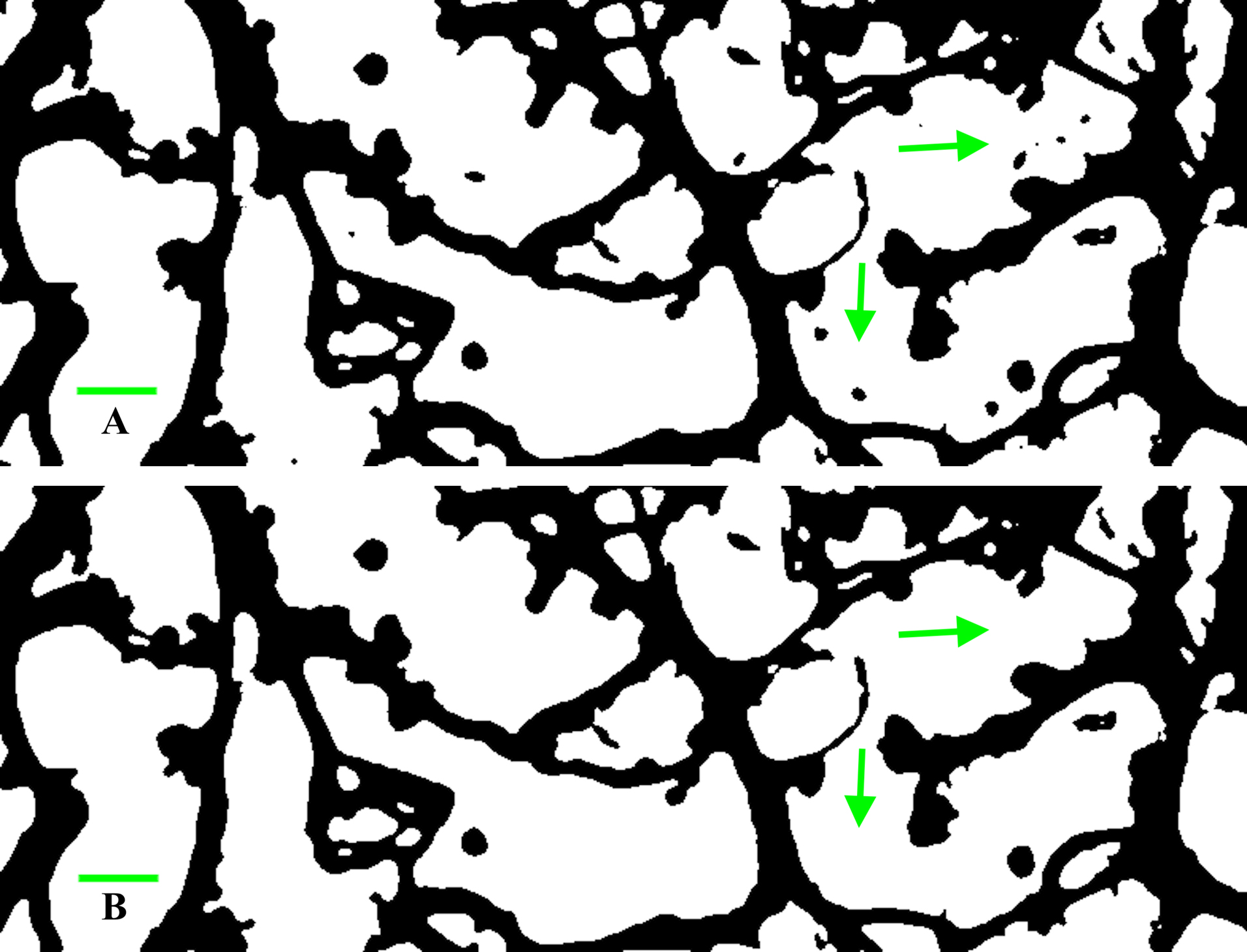
Figure 9. Representative image before (A) and after (B) the filtering process, removing objects smaller than 100 µm2. Arrows point to some areas that were cleared. Scale bar, 50 µm.
11. Use morphological filters (Plugins > MorphoLibJ > Morphological Filters) to further filter the image to maintain the overall structure of the vasculature.
Note: This is useful for smoothening the borders of the vascular structure and dealing with holes, but it can significantly impact the morphology when holes and branches are changed or eliminated.
a. Opening: Eroding and then dilating the binary image by a set number of pixels using an “element.” In other words, the shape and size of the brush that will scrub over the image. This is useful for smoothening shape borders, pruning thin unwanted branches, or widening gaps.
b. Closing: Dilating then eroding using a set element. Useful for filling holes and gaps and smoothing borders.
c. Filters can be used in combination/series to great effect (Figure 10).
i. Opening and closing operation with a square shape and pixel size of 1–2 is typically used.
ii. Directional morphological filters may be better at highlighting thin structures, since the elements are lines rather than blocks.
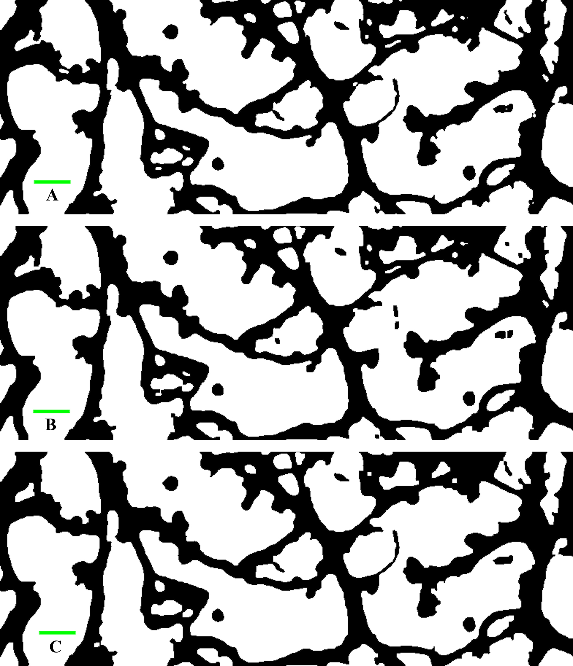
Figure 10. Examples of the effect of morphological filters from the original image (A) and after an opening filter (B) or closing filter (C). Scale bars, 50 µm.
G. Measure vessel density, lacunarity, and tortuosity
1. Based on the binary image, calculate the vessel density, Db, and Lac.
2. Plugins > BoneJ > Fraction > Area/volume fraction.
3. Plugins > MorphoLibJ > Analyze > Average Thickness.
4. Fractal analysis
a. Plugins > Fractal Analysis > FracLac. In the window, click the BC box for box-counting dimension, set the settings, click Ok, then click Scan.
b. Settings: Default except for: Lock white background, max grid size of 30 pixels, and regression graphic option checked.
c. Take the average Db (D̅ = ∑D₍ɢ₎/Ǥɴ∀ɢ∈Ǥ for Dʙ) and the lacunarity (L) = ∑Λ₍ɢ₎/Ǥɴ∀ɢ∈Ǥ
H. Skeletonization
1. Collapsing down the structure in the binary image so that all that is left is the connected centerlines of all the structures (Figure 11).
2. Plugins > Skeleton > Skeletonize (2D/3D)
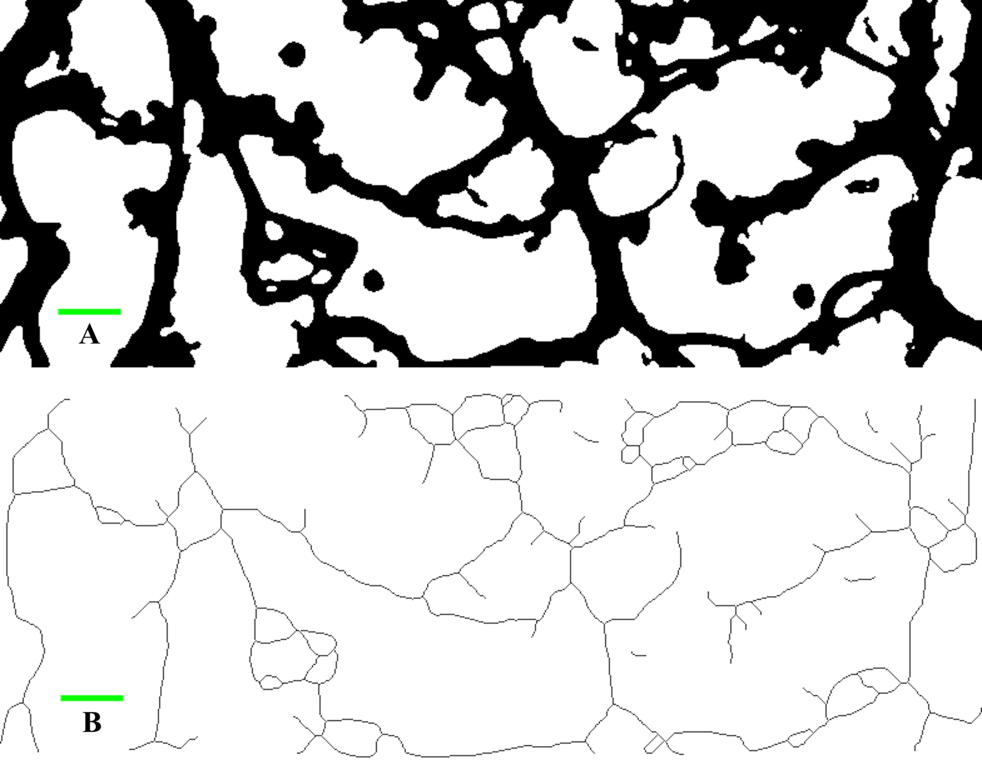
Figure 11. Representative image demonstrating the effect before (A) and after (B) skeletonization. Scale bar, 50 µm.
I. Measure branch length and number of branch points
1. Based on the skeleton, measure the average branch length and number of branches, junctions, and triple points.
2. Plugins > BoneJ > Analyze Skeleton (no pruning, nothing selected).
J. CC counting
1. Using the multi-point selection tool, mark and count each CC in the ROI images. CCs are roughly spherical bulbs of cells budding off vessels (Figure 12).
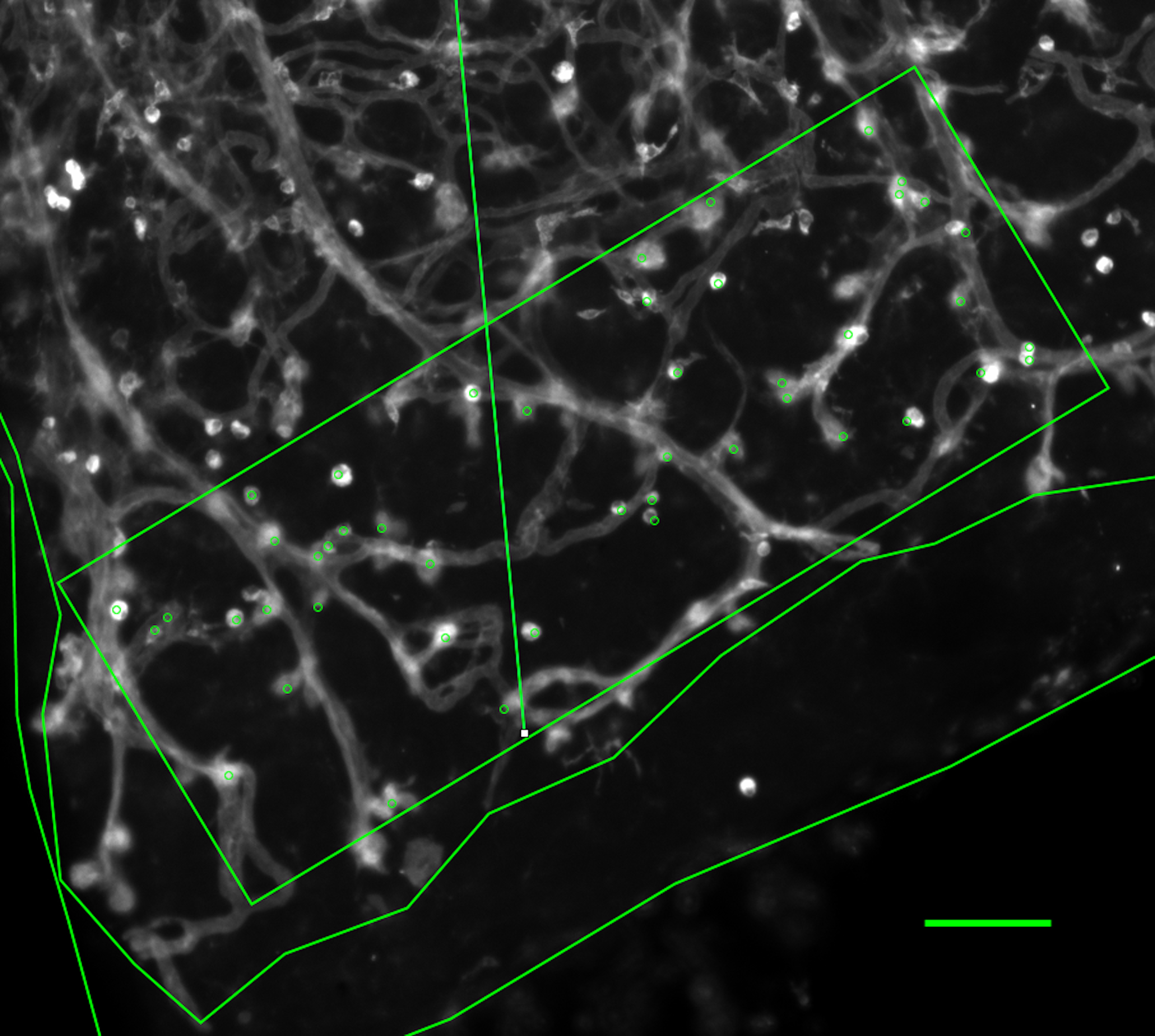
Figure 12. Cell clusters (CCs) are marked for counting in a region of interest (ROI). Scale bar, 100 µm.
2. Measure the overlay and take the total number of point entries.
K. Grading areas of vascular disorganization
1. Open the original retina image.
2. Outline the areas of vasculature disorganization using the polygon selection tool and measure the area similar to the methods of the total vascularized area noted above (Figures 13 and 14).
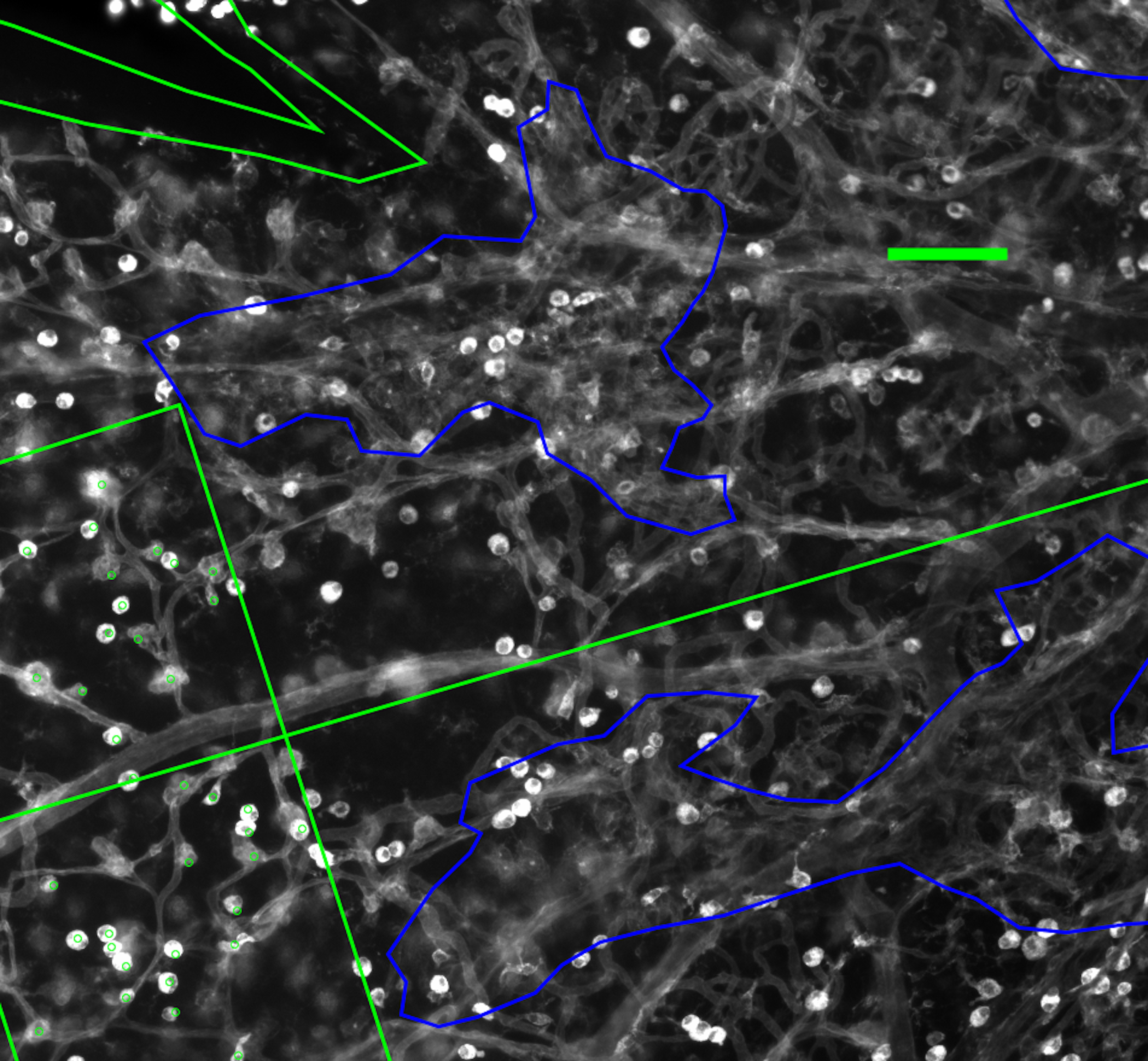
Figure 13. Example Grade 1 mesh outlined in blue. Grade 1 is an area with significant noise where vessels appear to be fused together but there is still some ordered structure. Scale bar, 100 µm.
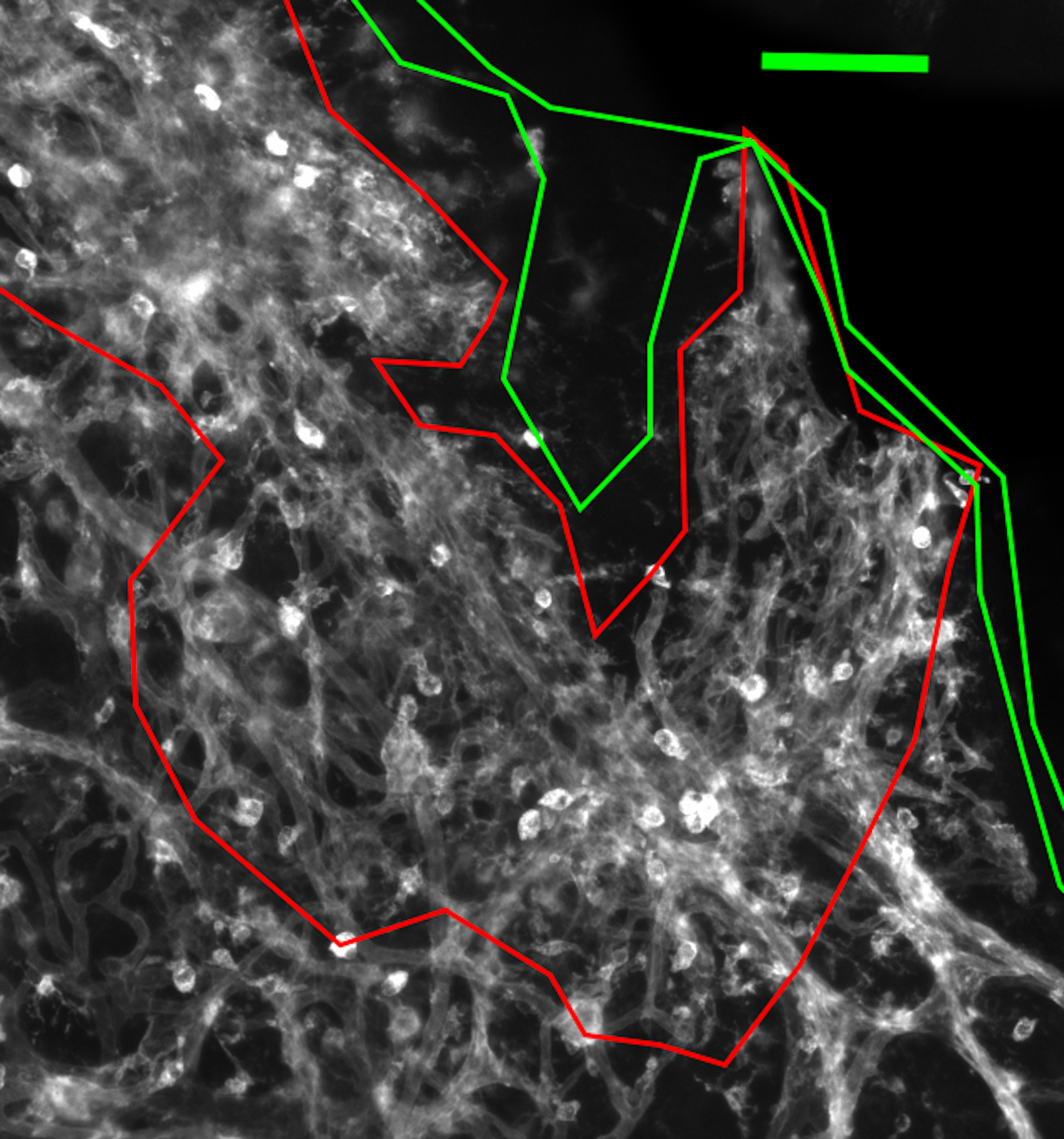
Figure 14. Example Grade 2 mesh outlined in red. Grade 2 is an area with significant noise that is an almost completely disordered mess of endothelial cells. The occasional defined vessel is not enough to classify it as Grade 1. Scale bar, 100 µm.
L. Summary
1. At the end of the analysis, you will have images of the whole retina flat mount (Figure 15), the different ROIs, the binary ROIs, the skeleton ROIs, and the FracLac outputs.
2. Measurement generated by the workflow (Figure 16):
a. Retinal area (μm2) and vascularized area/fraction (ratio).
b. Percent areas of Grade 1 and 2 meshes (%).
c. CC count of ROIs (count).
d. Vessel density (ratio).
e. Vessel average branch length and diameter (μm).
f. Number of junctions and triple points (count).
g. Db and lacunarity (unitless).
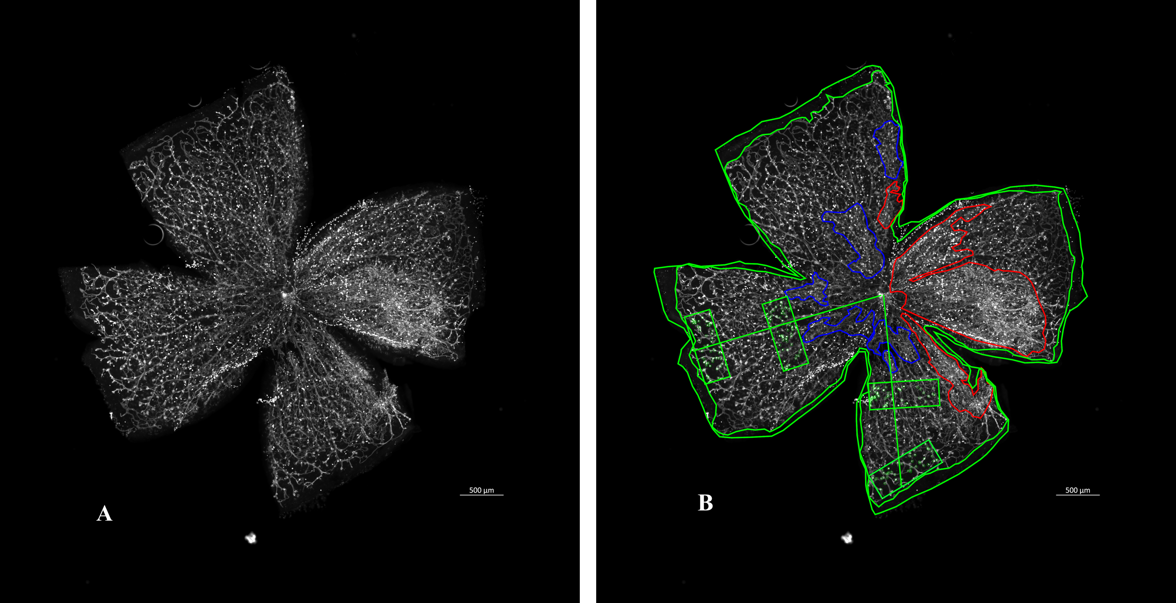
Figure 15. Whole retina flat mount image of the FZD4 mouse model. (A) Before and (B) after total retina and vascularized area, Grade 1 and 2 meshes (blue and red, respectively), periphery and mid-periphery 300 × 800 µm regions of interest (ROIs), and cell clusters (CCs) are outlined and labeled. Scale bar, 500 µm.
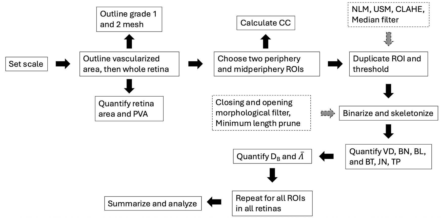
Figure 16. Workflow diagram for the digital image analysis of FZD4 models and wild-type (WT) controls. Abbreviations: NLM, non-local means; USM, unsharp mask; CLAHE, contrast-limited adaptive histogram equalization; CC, cell cluster count; VD, vessel density; BN, number of branches; BT, branch thickness; BL, branch length; JN, number of junctions; TP, number of triple points; Λ, lacunarity; DB, box-counting fractal dimension; ROI, region of interest.
Validation of protocol
This protocol has been used and validated in the following research article:
Feridooni et al. [72] Sphingosine-1-phosphate receptor 2 inhibition ameliorates familial exudative vitreoretinopathy models. Journal of Biological Chemistry (Figures 2–5).
General notes and troubleshooting
General notes
1. Not all tools should be used all the time, and each image requires different degrees of enhancement, filtering, etc. The goal is to get an accurate representation of the vascular structure; thus, we recommend the application of our protocol according to your best judgment for the highest quality data for your purposes. For this reason, we do not prescribe specific settings for each parameter as the image is processed.
2. Always save after every major step. There is no reliable undo or redo button in FIJI. It is important to save the final versions of selections, binary, and skeleton images. ImageJ guides for basic functions are available at https://imagej.nih.gov/ij/docs/guide/ and https://imagej.net (New ImageJ Wiki).
3. For minimum length prune, take the script listed on the Analyze Skeleton page and save it as a plugin. Instructions on how to do so are here available at https://imagej.net/scripting/.
4. Batch analysis in FIJI and FracLac can be incorporated depending on the level of automation (macros) you implement.
5. You can easily create your own macro by using the Macro Recorder tool or scripting to automate any steps to save time (https://imagej.net/scripting/macro).
6. Retinal vasculature labeling, image acquisition, and quality would evidently impact results. Our full method is presented in our validation study [73], and including this methodology is beyond the scope of this paper, as it is focused on computational analysis. To briefly summarize, retinal whole mounts were stained with Alexa Fluor 594–conjugated GS-IB4 lectin to visualize the vascular endothelium, as previously described [73–77]. Images were acquired at 10× magnification using a Zeiss Axio Imager Z2 microscope equipped with a motorized digital stage and MosaiX software in Axiovision 4.8, with all samples imaged under identical acquisition settings.
Troubleshooting
Problem 1: Unexpected error.
Possible cause: Using old versions of plugins, or an aspect of the underlying code is causing an error.
Solutions: Refer to https://imagej.net/plugins/updater for more details on how to regularly update all plugins and FIJI. Get in contact with the broader image analysis and FIJI development community on https://forum.image.sc for custom solutions and direct contact with developers.
Acknowledgments
This work was supported by a Canadian Institutes of Health Research grant to CRM (Grant #SOP-159230). The protocol was first published in [72].
Competing interests
The authors declare no conflicts of interest.
Ethical considerations
Mouse flat mounts for computational analysis were performed in accordance with the Guide to Care and Use of Experimental Animals by the Canadian Council on Animal Care and approved by the Research Ethics Board for Laboratory Animal Research at Dalhousie University.
References
- Heath Jeffery, R. C., Mukhtar, S. A., McAllister, I. L., Morgan, W. H., Mackey, D. A. and Chen, F. K. (2021). Inherited retinal diseases are the most common cause of blindness in the working-age population in Australia. Ophthalmic Genet. 42(4): 431–439. https://doi.org/10.1080/13816810.2021.1913610
- Liew, G., Michaelides, M. and Bunce, C. (2014). A comparison of the causes of blindness certifications in England and Wales in working age adults (16–64 years), 1999–2000 with 2009–2010. BMJ Open. 4(2): e004015. https://doi.org/10.1136/bmjopen-2013-004015
- Lim, H. W., Pershing, S., Moshfeghi, D. M., Heo, H., Haque, M. E., Lambert, S. R., Pershing, S., Hyman, L., Haller, J. A., Lee, A. Y., et al. (2023). Causes of Childhood Blindness in the United States Using the IRIS® Registry (Intelligent Research in Sight). Ophthalmology. 130(9): 907–913. https://doi.org/10.1016/j.ophtha.2023.04.004
- Kour, V., Swain, J., Singh, J., Singh, H. and Kour, H. (2024). A Review on Diabetic Retinopathy. Curr Diabetes Rev. 20(6): e201023222418. https://doi.org/10.2174/0115733998253672231011161400
- Mishra, S., Vishwakarma, P. K., Tripathi, M., Ojha, S. and Tripathi, S. M. (2024). Diabetic Retinopathy: Clinical Features, Risk Factors, and Treatment Options. Curr Diabetes Rev. 20(7): e2174/0115733998252551231018080419. https://doi.org/10.2174/0115733998252551231018080419
- Senjam, S. S. (2024). Diabetes and diabetic retinopathy: the growing public health concerns in India. Lancet Global Health. 12(5): e727–e728. https://doi.org/10.1016/s2214-109x(24)00075-5
- Yang, Y. M., Lu, Y. M. and Hsu, C. H. (2024). Limitations of Assessing Barriers in Diabetic Retinopathy Screening. JAMA Ophthalmol. 142(5): 491. https://doi.org/10.1001/jamaophthalmol.2024.0317
- Binenbaum, G. (2024). Is Artificial Intelligence for Retinopathy of Prematurity Ready to Go?. JAMA Ophthalmol. 142(4): 335. https://doi.org/10.1001/jamaophthalmol.2024.0218
- Ells, A., Guernsey, D. L., Wallace, K., Zheng, B., Vincer, M., Allen, A., Ingram, A., DaSilva, O., Siebert, L., Sheidow, T., et al. (2010). Severe retinopathy of prematurity associated withFZD4mutations. Ophthalmic Genet. 31(1): 37–43. https://doi.org/10.3109/13816810903479834
- García, H., Villasis-Keever, M. A., Zavala-Vargas, G., Bravo-Ortiz, J. C., Pérez-Méndez, A. and Escamilla-Núñez, A. (2024). Global Prevalence and Severity of Retinopathy of Prematurity over the Last Four Decades (1985–2021): A Systematic Review and Meta-Analysis. Arch Med Res. 55(2): 102967. https://doi.org/10.1016/j.arcmed.2024.102967
- Kubota, H., Fukushima, Y., Kawasaki, R., Endo, T., Hatsukawa, Y., Ineyama, H., Hirata, K., Hirano, S., Wada, K., Nishida, K., et al. (2024). Continuous oxygen saturation and risk of retinopathy of prematurity in a Japanese cohort. Br J Ophthalmol. 108(9): 1275–1280. https://doi.org/10.1136/bjo-2023-324225
- Lee, C. C., Chiang, M. C., Chu, S. M., Wu, W. C., Ho, M. C. and Lien, R. (2024). Clinical Risk Factors for Retinopathy of Prematurity Reactivation after Intravitreal Antivascular Endothelial Growth Factor Injection. J Pediatr. 273: 113913. https://doi.org/10.1016/j.jpeds.2024.113913
- Chen, Z. Y., Battinelli, E., Fielder, A., Bundey, S., Sims, K., Breakefield, X. and Craig, I. (1993). A mutation in the Norrie disease gene (NDP) associated with X–linked familial exudative vitreoretinopathy. Nat Genet. 5(2): 180–183. https://doi.org/10.1038/ng1093-180
- Hoem, G., Pastore, A., Bratland, E., Christoffersen, T., Stornaiuolo, M. and Douzgou, S. (2024). Severe isolated exudative vitreoretinopathy caused by biallelic FZD4 variants. Clin Genet. 105(6): 661–665. https://doi.org/10.1111/cge.14499
- Hu, H., Xiao, X., Li, S., Jia, X., Guo, X. and Zhang, Q. (2015). KIF11mutations are a common cause of autosomal dominant familial exudative vitreoretinopathy. Br J Ophthalmol. 100(2): 278–283. https://doi.org/10.1136/bjophthalmol-2015-306878
- Lai, M. B., Zhang, C., Shi, J., Johnson, V., Khandan, L., McVey, J., Klymkowsky, M. W., Chen, Z. and Junge, H. J. (2017). TSPAN12 Is a Norrin Co-receptor that Amplifies Frizzled4 Ligand Selectivity and Signaling. Cell Rep. 19(13): 2809–2822. https://doi.org/10.1016/j.celrep.2017.06.004
- Lu, J., Huang, L., Sun, L., Li, S., Zhang, Z., Jiang, Z., Li, J. and Ding, X. (2022). FZD4 in a Large Chinese Population With Familial Exudative Vitreoretinopathy: Molecular Characteristics and Clinical Manifestations. Invest Ophthalmol Vis Sci. 63(4): 7. https://doi.org/10.1167/iovs.63.4.7
- Luhmann, U. F. O., Neidhardt, J., Kloeckener‐Gruissem, B., Schäfer, N. F., Glaus, E., Feil, S. and Berger, W. (2008). Vascular changes in the cerebellum of Norrin /Ndph knockout mice correlate with high expression of Norrin and Frizzled‐4. Eur J Neurosci. 27(10): 2619–2628. https://doi.org/10.1111/j.1460-9568.2008.06237.x
- Ngo, M. H., Borowska-Fielding, J., Heathcote, G., Nejat, S., Kelly, M. E., McMaster, C. R. and Robitaille, J. M. (2016). Fzd4 Haploinsufficiency Delays Retinal Revascularization in the Mouse Model of Oxygen Induced Retinopathy. PLoS One. 11(8): e0158320. https://doi.org/10.1371/journal.pone.0158320
- Park, H., Yamamoto, H., Mohn, L., Ambühl, L., Kanai, K., Schmidt, I., Kim, K. P., Fraccaroli, A., Feil, S., Junge, H. J., et al. (2019). Integrin-linked kinase controls retinal angiogenesis and is linked to Wnt signaling and exudative vitreoretinopathy. Nat Commun. 10(1): e1038/s41467–019–13220–3. https://doi.org/10.1038/s41467-019-13220-3
- Poulter, J. A., Ali, M., Gilmour, D. F., Rice, A., Kondo, H., Hayashi, K., Mackey, D. A., Kearns, L. S., Ruddle, J. B., Craig, J. E., et al. (2016). Mutations in TSPAN12 Cause Autosomal-Dominant Familial Exudative Vitreoretinopathy. Am J Hum Genet. 98(3): 592. https://doi.org/10.1016/j.ajhg.2016.02.017
- Rao, F. Q., Cai, X. B., Cheng, F. F., Cheng, W., Fang, X. L., Li, N., Huang, X. F., Li, L. H. and Jin, Z. B. (2017). Mutations in LRP5 , FZD4 , TSPAN12 , NDP , ZNF408 , or KIF11 Genes Account for 38.7% of Chinese Patients With Familial Exudative Vitreoretinopathy. Invest Ophthalmol Vis Sci. 58(5): 2623. https://doi.org/10.1167/iovs.16-21324
- Robitaille, J., MacDonald, M. L., Kaykas, A., Sheldahl, L. C., Zeisler, J., Dubé, M. P., Zhang, L. H., Singaraja, R. R., Guernsey, D. L., Zheng, B., et al. (2002). Mutant frizzled-4 disrupts retinal angiogenesis in familial exudative vitreoretinopathy. Nat Genet. 32(2): 326–330. https://doi.org/10.1038/ng957
- Robitaille, J. M., Gillett, R. M., LeBlanc, M. A., Gaston, D., Nightingale, M., Mackley, M. P., Parkash, S., Hathaway, J., Thomas, A., Ells, A., et al. (2014). Phenotypic Overlap Between Familial Exudative Vitreoretinopathy and Microcephaly, Lymphedema, and Chorioretinal Dysplasia Caused byKIF11Mutations. JAMA Ophthalmol. 132(12): 1393. https://doi.org/10.1001/jamaophthalmol.2014.2814
- van der Ende, S. R., Meyers, B. S., Capasso, J. E., Sasongko, M., Yonekawa, Y., Pihlblad, M., Huey, J., Bedoukian, E. C., Krantz, I. D., Ngo, M. H., et al. (2022). Severe Familial Exudative Vitreoretinopathy, Congenital Hearing Loss, and Developmental Delay in a Child With Biallelic Variants in FZD4. JAMA Ophthalmol. 140(9): 889. https://doi.org/10.1001/jamaophthalmol.2022.2914
- Wang, Y., Smallwood, P. M., Williams, J. and Nathans, J. (2020). A mouse model for kinesin family member 11 (Kif11)-associated familial exudative vitreoretinopathy. Hum Mol Genet. 29(7): 1121–1131. https://doi.org/10.1093/hmg/ddaa018
- Xu, Q., Wang, Y., Dabdoub, A., Smallwood, P. M., Williams, J., Woods, C., Kelley, M. W., Jiang, L., Tasman, W., Zhang, K. and Nathans, J. (2004). Vascular development in the retina and inner ear: control by Norrin and Frizzled-4, a high-affinity ligand-receptor pair. Cell. 116(6):883–95. https://doi.org/10.1016/s0092-8674(04)00216-8
- Yang, M., Li, S., Huang, L., Zhao, R., Dai, E., Jiang, X., He, Y., Lu, J., Peng, L., Liu, W., et al. (2022). CTNND1 variants cause familial exudative vitreoretinopathy through the Wnt/cadherin axis. JCI Insight. 7(14): e158428. https://doi.org/10.1172/jci.insight.158428
- Zhu, X., Yang, M., Zhao, P., Li, S., Zhang, L., Huang, L., Huang, Y., Fei, P., Yang, Y., Zhang, S., et al. (2021). Catenin α 1 mutations cause familial exudative vitreoretinopathy by overactivating Norrin/β-catenin signaling. J Clin Invest. 131(6): e1172/jci139869. https://doi.org/10.1172/jci139869
- Junge, H. J., Yang, S., Burton, J. B., Paes, K., Shu, X., French, D. M., Costa, M., Rice, D. S. and Ye, W. (2009). TSPAN12 Regulates Retinal Vascular Development by Promoting Norrin- but Not Wnt-Induced FZD4/β-Catenin Signaling. Cell. 139(2): 299–311. https://doi.org/10.1016/j.cell.2009.07.048
- Paes, K. T., Wang, E., Henze, K., Vogel, P., Read, R., Suwanichkul, A., Kirkpatrick, L. L., Potter, D., Newhouse, M. M., Rice, D. S., et al. (2011). Frizzled 4 Is Required for Retinal Angiogenesis and Maintenance of the Blood-Retina Barrier. Invest Ophthalmol Vis Sci. 52(9): 6452. https://doi.org/10.1167/iovs.10-7146
- Wang, Y., Rattner, A., Zhou, Y., Williams, J., Smallwood, P. M. and Nathans, J. (2012). Norrin/Frizzled4 Signaling in Retinal Vascular Development and Blood Brain Barrier Plasticity. Cell. 151(6): 1332–1344. https://doi.org/10.1016/j.cell.2012.10.042
- Ye, X., Wang, Y., Cahill, H., Yu, M., Badea, T. C., Smallwood, P. M., Peachey, N. S. and Nathans, J. (2009). Norrin, Frizzled-4, and Lrp5 Signaling in Endothelial Cells Controls a Genetic Program for Retinal Vascularization. Cell. 139(2): 285–298. https://doi.org/10.1016/j.cell.2009.07.047
- Zuercher, J., Fritzsche, M., Feil, S., Mohn, L. and Berger, W. (2012). Norrin stimulates cell proliferation in the superficial retinal vascular plexus and is pivotal for the recruitment of mural cells. Hum Mol Genet. 21(12): 2619–2630. https://doi.org/10.1093/hmg/dds087
- Connor, K. M., Krah, N. M., Dennison, R. J., Aderman, C. M., Chen, J., Guerin, K. I., Sapieha, P., Stahl, A., Willett, K. L., Smith, L. E. H., et al. (2009). Quantification of oxygen-induced retinopathy in the mouse: a model of vessel loss, vessel regrowth and pathological angiogenesis. Nat Protoc. 4(11): 1565–1573. https://doi.org/10.1038/nprot.2009.187
- Dellian, M., Witwer, B. P., Salehi, H. A., Yuan, F. and Jain, R. K. (1996). Quantitation and Physiological Characterization of Angiogenic Vessels in Mice. American Journal of Pathology. 149(1): 13. https://pubmed.ncbi.nlm.nih.gov/8686763/
- Carpentier, G., Berndt, S., Ferratge, S., Rasband, W., Cuendet, M., Uzan, G. and Albanese, P. (2020). Angiogenesis Analyzer for ImageJ — A comparative morphometric analysis of “Endothelial Tube Formation Assay” and “Fibrin Bead Assay”. Sci Rep. 10(1): e1038/s41598–020–67289–8. https://doi.org/10.1038/s41598-020-67289-8
- Corliss, B. A., Doty, R. W., Mathews, C., Yates, P. A., Zhang, T. and Peirce, S. M. (2020). REAVER: A program for improved analysis of high‐resolution vascular network images. Microcirculation. 27(5): e12618. https://doi.org/10.1111/micc.12618
- Elfarnawany, M. H. (2015). Signal Processing Methods for Quantitative Power Doppler Microvascular Angiography. The University of Western Ontario. 192.
- Niemisto, A., Dunmire, V., Yli-Harja, O., Wei Zhang. and Shmulevich, I. (2005). Robust quantification of in vitro angiogenesis through image analysis. IEEE Trans Med Imaging. 24(4): 549–553. https://doi.org/10.1109/tmi.2004.837339
- Seaman, M. E., Peirce, S. M. and Kelly, K. (2011). Rapid Analysis of Vessel Elements (RAVE): A Tool for Studying Physiologic, Pathologic and Tumor Angiogenesis. PLoS One. 6(6): e20807. https://doi.org/10.1371/journal.pone.0020807
- Yim-lui Cheung, C., Hsu, W., Lee, M. L., Wang, J. J., Mitchell, P., Peter Lau, Q., Hamzah, H., Ho, M. and Wong, T. Y. (2010). A New Method to Measure Peripheral Retinal Vascular Caliber over an Extended Area. Microcirculation : no–no. https://doi.org/10.1111/j.1549-8719.2010.00048.x
- Zudaire, E., Gambardella, L., Kurcz, C. and Vermeren, S. (2011). A Computational Tool for Quantitative Analysis of Vascular Networks. PLoS One. 6(11): e27385. https://doi.org/10.1371/journal.pone.0027385
- Schneider, C. A., Rasband, W. S. and Eliceiri, K. W. (2012). NIH Image to ImageJ: 25 years of image analysis. Nat Methods. 9(7): 671–675. https://doi.org/10.1038/nmeth.2089
- Hotaling, N. A., Bharti, K., Kriel, H. and Simon, C. G. (2015). DiameterJ: A validated open source nanofiber diameter measurement tool. Biomaterials. 61: 327–338. https://doi.org/10.1016/j.biomaterials.2015.05.015
- Simon, C. and Hotaling. (2019). DiameterJ. (Accessed February 9, 2026, at https://www.nist.gov/mml/bbd/biomaterials/diameterj)
- Niemisto, A., Dunmire, V., Yli-Harja, O., Wei Zhang. and Shmulevich, I. (2005). Robust quantification of in vitro angiogenesis through image analysis. IEEE Trans Med Imaging. 24(4): 549–553. https://doi.org/10.1109/tmi.2004.837339
- Arganda‐Carreras, I., Fernández‐González, R., Muñoz‐Barrutia, A. and Ortiz‐De‐Solorzano, C. (2010). 3D reconstruction of histological sections: Application to mammary gland tissue. Microsc Res Tech. 73(11): 1019–1029. https://doi.org/10.1002/jemt.20829
- Domander, R., Felder, A. A. and Doube, M. (2021). BoneJ2 - refactoring established research software. Wellcome Open Res. 6: 37. https://doi.org/10.12688/wellcomeopenres.16619.2
- Chu, Z., Lin, J., Gao, C., Xin, C., Zhang, Q., Chen, C. L., Roisman, L., Gregori, G., Rosenfeld, P. J., Wang, R. K., et al. (2016). Quantitative assessment of the retinal microvasculature using optical coherence tomography angiography. J Biomed Opt. 21(6): 066008. https://doi.org/10.1117/1.jbo.21.6.066008
- Li, L., Ikram, M. K. and Wong, T. Y. (2015). Retinal vascular imaging in early life: insights into processes and risk of cardiovascular disease. J Physiol. 594(8): 2175–2203. https://doi.org/10.1113/jp270947
- Ţălu, Ş. (2013). Characterization of retinal vessel networks in human retinal imagery using quantitative descriptors. Human and Veterinary Medicine. 5: 52–57.
- Corliss, B. A., Mathews, C., Doty, R., Rohde, G. and Peirce, S. M. (2019). Methods to label, image, and analyze the complex structural architectures of microvascular networks. Microcirculation 26(5): e12520. https://doi.org/10.1111/micc.12520
- Dougherty, G., Johnson, M. J. and Wiers, M. D. (2009). Measurement of retinal vascular tortuosity and its application to retinal pathologies. Med Biol Eng Comput. 48(1): 87–95. https://doi.org/10.1007/s11517-009-0559-4
- Khansari, M. M., O’Neill, W., Lim, J. and Shahidi, M. (2017). Method for quantitative assessment of retinal vessel tortuosity in optical coherence tomography angiography applied to sickle cell retinopathy. Biomed Opt Express. 8(8): 3796. https://doi.org/10.1364/boe.8.003796
- Family, F., Masters, B. R. and Platt, D. E. (1989). Fractal pattern formation in human retinal vessels. Physica D. 38: 98–103. https://doi.org/10.1016/0167-2789(89)90178-4
- Lemmens, S., Devulder, A., Van Keer, K., Bierkens, J., De Boever, P. and Stalmans, I. (2020). Systematic Review on Fractal Dimension of the Retinal Vasculature in Neurodegeneration and Stroke: Assessment of a Potential Biomarker. Front Neurosci. 14: e00016. https://doi.org/10.3389/fnins.2020.00016
- Popovic, N., Lipovac, M., Radunovic, M., Ugarte, J., Isusquiza, E., Beristain, A., Moreno, R., Aranjuelo, N. and Popovic, T. (2019). Fractal characterization of retinal microvascular network morphology during diabetic retinopathy progression. Microcirculation. 26(4): e12531. https://doi.org/10.1111/micc.12531
- Sijilmassi, O., López Alonso, J. M., Del Río Sevilla, A. and Barrio Asensio, M. d. C. (2020). Multifractal analysis of embryonic eye structures from female mice with dietary folic acid deficiency. Part I: Fractal dimension, lacunarity, divergence, and multifractal spectrum. Chaos Soliton Fract. 138: 109885. https://doi.org/10.1016/j.chaos.2020.109885
- Sijilmassi, O., López Alonso, J. M., Del Río Sevilla, A. and Barrio Asensio, M. d. C. (2020). Multifractal analysis of embryonic eye tissues from female mice with folic acid deficiency. Part II: Local Connected Fractal Dimension Analysis. Chaos, Solitons & Fractals 138: 109887. https://doi.org/10.1016/j.chaos.2020.109887
- Yu, S. and Lakshminarayanan, V. (2021). Fractal Dimension and Retinal Pathology: A Meta-Analysis. Appl Sci. 11(5): 2376. https://doi.org/10.3390/app11052376
- Karperien, A. L. and Jelinek, H. F. (2016). Morphology and Fractal-Based Classifications of Neurons and Microglia. Di Ieva, A. (Ed.) The Fractal Geometry of the Brain. Springer New York, 91–108. https://doi.org/10.1007/978-1-4939-3995-4_6
- Liebovitch, L. S. and Toth, T. (1989). A fast algorithm to determine fractal dimensions by box counting. Phys Lett A. 141: 386–390. https://doi.org/10.1016/0375-9601(89)90854-2
- Huang, F., Dashtbozorg, B., Zhang, J., Bekkers, E., Abbasi-Sureshjani, S., Berendschot, T. T. J. M. and ter Haar Romeny, B. M. (2016). Reliability of Using Retinal Vascular Fractal Dimension as a Biomarker in the Diabetic Retinopathy Detection. J Ophthalmol. 2016: 1–13. https://doi.org/10.1155/2016/6259047
- Landini, G., Murray, P. I. and Missonf, G. P. (1995). Local Connected Fractal Dimensions and Lacunarity Analyses of 60° Fluorescein Angiograms. Investigative Ophthalmology. 36(13): 7. https://pubmed.ncbi.nlm.nih.gov/7499097/
- Voss, R. F. and Wyatt, J. C. Y. (1993). Multifractals and the Local Connected Fractal Dimension. Crilly, A. J., Earnshaw, R. A. and Jones, H. (Eds.) Applications of Fractals and Chaos. Springer Berlin Heidelberg. 171–192. https://doi.org/10.1007/978-3-642-78097-4_11
- Chaudhuri, B. and Sarkar, N. (1995). Texture segmentation using fractal dimension. IEEE Trans Pattern Anal Mach Intell. 17(1): 72–77. https://doi.org/10.1109/34.368149
- Lopes, R. and Betrouni, N. (2009). Fractal and multifractal analysis: A review. Med Image Anal. 13(4): 634–649. https://doi.org/10.1016/j.media.2009.05.003
- Mookiah, M. R. K., Tan, J. H., Chua, C. K., Ng, E. Y. K., Laude, A. and Tong, L. (2015). Automated Characterization and Detection of Diabetic Retinopathy Using Texture Measures. J Mech Med Biol. 15(4): 1550045. https://doi.org/10.1142/s0219519415500451
- Xue, S., Jiang, X. and Duan, J. (2017). A new box-counting method for image fractal dimension estimation. 2017 3rd IEEE International Conference on Computer and Communications (ICCC). IEEE. 1786–1791. https://doi.org/10.1109/ICIP.2006.313005
- Sandau, K. and Kurz, H. (1997). Measuring fractal dimension and complexity — an alternative approach with an application. J Microsc. 186(2): 164–176. https://doi.org/10.1046/j.1365-2818.1997.1270685.x
- Feridooni, H. A., Fody, R., Tavasoli, M., Alkandari, M., van der Ende, S., Nader, M., Robitaille, J. M. and McMaster, C. R. (2026). Sphingosine-1-phosphate receptor 2 inhibition ameliorates familial exudative vitreoretinopathy models. J Biol Chem. 302(2): 111107. https://doi.org/10.1016/j.jbc.2025.111107
- Wang, Y., Rattner, A., Zhou, Y., Williams, J., Smallwood, P. M. and Nathans, J. (2012). Norrin/Frizzled4 Signaling in Retinal Vascular Development and Blood Brain Barrier Plasticity. Cell. 151(6): 1332–1344. https://doi.org/10.1016/j.cell.2012.10.042
- Xu, Q., Wang, Y., Dabdoub, A., Smallwood, P. M., Williams, J., Woods, C., Kelley, M. W., Jiang, L., Tasman, W., Zhang, K., et al. (2004). Vascular Development in the Retina and Inner Ear: Control by Norrin and Frizzled-4, a High-Affinity Ligand-Receptor Pair. Cell. 116(6), 883–895. https://doi.org/10.1016/S0092-8674(04)00216-8
- Ye, X., Wang, Y., Cahill, H., Yu, M., Badea, T. C., Smallwood, P. M., Peachey, N. S. and Nathans, J. (2009). Norrin, Frizzled-4, and Lrp5 Signaling in Endothelial Cells Controls a Genetic Program for Retinal Vascularization. Cell. 139(2): 285–298. https://doi.org/10.1016/j.cell.2009.07.047
- Ngo, M. H., Borowska-Fielding, J., Heathcote, G., Nejat, S., Kelly, M. E., McMaster, C. R. and Robitaille, J. M. (2016). Fzd4 Haploinsufficiency Delays Retinal Revascularization in the Mouse Model of Oxygen Induced Retinopathy. PLoS One. 11(8): e0158320. https://doi.org/10.1371/journal.pone.0158320
- Adini, I. and Ghosh, K. (2015). Mouse Retinal Whole Mounts and Quantification of Vasculature Protocol. Bio Protoc. 5(15): e1546. https://doi.org/10.21769/bioprotoc.1546
Article Information
Publication history
Received: Feb 12, 2026
Accepted: Apr 17, 2026
Available online: May 12, 2026
Published: Jun 5, 2026
Copyright
© 2026 The Author(s); This is an open access article under the CC BY license (https://creativecommons.org/licenses/by/4.0/).
How to cite
Readers should cite both the Bio-protocol article and the original research article where this protocol was used:
- Nader, M., Feridooni, H. A., Tavasoli, M., Van Der Ende, S., McMaster, C. R. and Robitaille, J. M. (2026). Computational Quantification of Mouse Retinal Vasculature Using ImageJ. Bio-protocol 16(11): e5705. DOI: 10.21769/BioProtoc.5705.
- Feridooni, H. A., Fody, R., Tavasoli, M., Alkandari, M., van der Ende, S., Nader, M., Robitaille, J. M. and McMaster, C. R. (2026). Sphingosine-1-phosphate receptor 2 inhibition ameliorates familial exudative vitreoretinopathy models. J Biol Chem. 302(2): 111107. https://doi.org/10.1016/j.jbc.2025.111107

 Download Citation in RIS Format
Category
Bioinformatics and Computational Biology
Neuroscience > Sensory and motor systems > Retina
Cell Biology > Tissue analysis > Histomorphology
Do you have any questions about this protocol?
Post your question to gather feedback from the community. We will also invite the authors of this article to respond.
 Post a Question


