- Protocols

- Articles and Issues
- For Authors
- About
- Become a Reviewer

Identifying and Characterizing Lipid-Binding Cavities in Lipid Transfer Proteins With CG-MD Simulations
(*contributed equally to this work) Published: Vol 15, Iss 24, Dec 20, 2025 DOI: 10.21769/BioProtoc.5558 Views: 688
Reviewed by: Anonymous reviewer(s)
Original research article
The authors used this protocol in:

Nov 2024
Advertisement


Protocol Collections
Comprehensive collections of detailed, peer-reviewed protocols focusing on specific topics


Abstract
Understanding how lipids interact with lipid transfer proteins (LTPs) is essential for uncovering their molecular mechanisms. Yet, many available LTP structures, particularly those thought to function as membrane bridges, lack detailed information on where their native lipid ligands are located. Computational strategies, such as docking or AI-methods, offer a valuable alternative to overcome this gap, but their effectiveness is often restricted by the inherent flexibility of lipid molecules and the lack of large training sets with structures of proteins bound to lipids. To tackle this issue, we introduce a reproducible computational pipeline that uses unbiased coarse-grained molecular dynamics (CG-MD) simulations on a free and open-source software (GROMACS) with the Martini 3 force-field. Starting from a configuration of a lipid in bulk solvent, we run CG-MD simulations and observe spontaneous binding of the lipid to the protein. We show that this protocol reliably identifies lipid-binding pockets in LTPs and, unlike docking methods, suggests potential entry routes for lipid molecules with no a priori knowledge other than the protein’s structure. We demonstrate the utility of this approach in investigating bridge LTPs whose internal lipid-binding positions remain unresolved. Altogether, our study provides a cost-effective, efficient, and accurate framework for mapping binding sites and entry pathways in diverse LTPs.
Key features
• Demonstrates the reliability of unbiased coarse-grain molecular dynamics (CG-MD) simulations with the Martini 3 force-field in identifying lipid-binding sites in lipid transfer proteins (LTPs).
• The protocol is straightforward to replicate, relying solely on freely available open-source software.
• Furthermore, it is computationally efficient, with most simulations completing within a few hours on a standalone GPU-accelerated workstation.
• As input, the user only needs to include the structure of the protein and select the lipid type to test.
Keywords: Coarse-grain MD simulationsGraphical overview
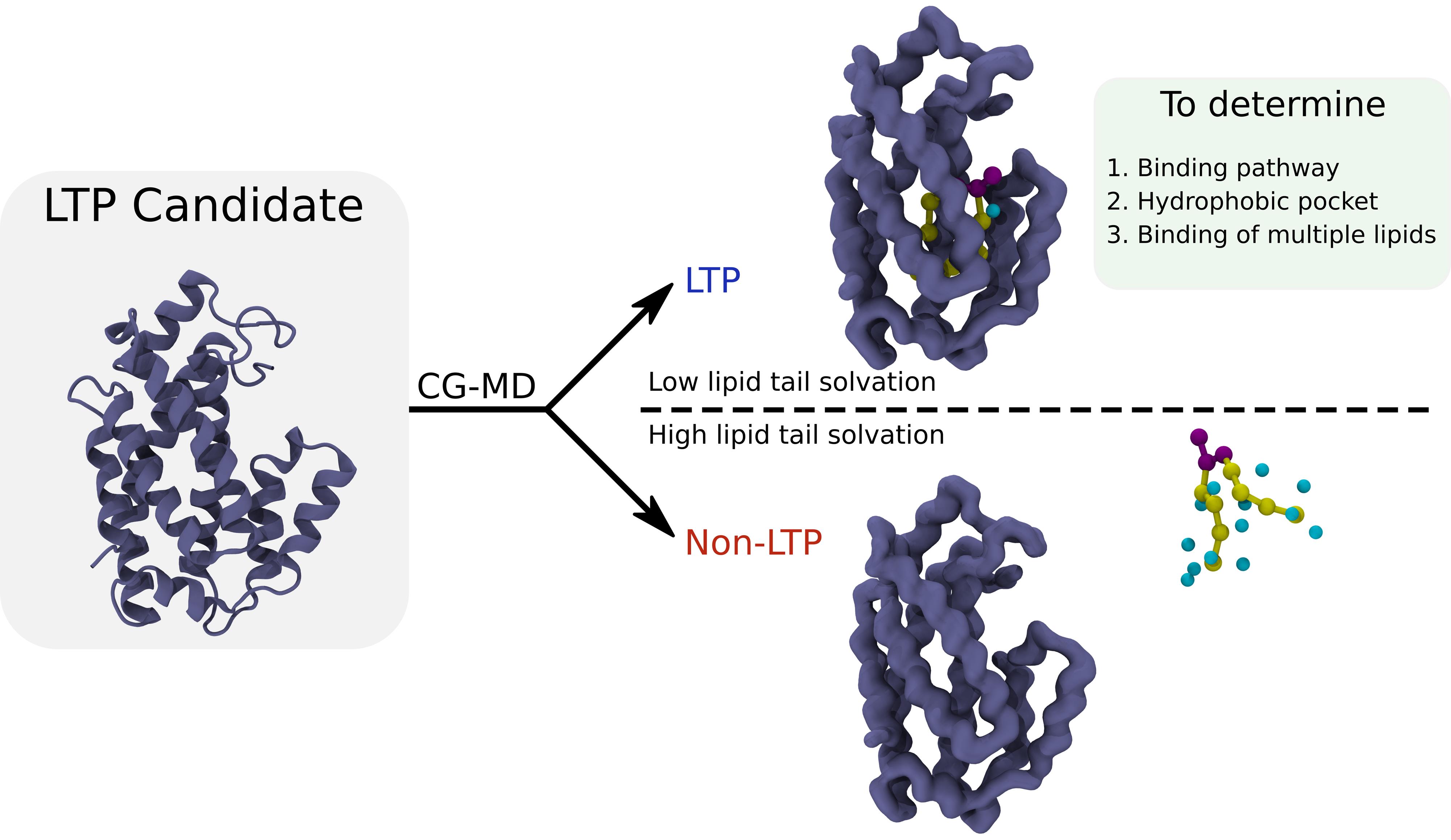
Coarse-grained molecular dynamics (CG-MD) simulations can identify the binding cavity of lipid transfer proteins. The protocol can also be used to characterize the lipid-binding cavity, as well as the binding pathway of the lipids. Further, it can be employed iteratively to study the binding of multiple lipids to the same cavity.
Background
Eukaryotic cells are compartmentalized into membrane-bound organelles, each defined by a unique lipid composition essential for its function. Preserving this lipid balance requires selective transport between organelles, mediated by both vesicular and non-vesicular mechanisms. A major class of mediators of non-vesicular lipid trafficking is lipid transfer proteins (LTPs), which encapsulate lipids in hydrophobic cavities and transfer them between membranes. In recent years, many new LTPs have been identified, highlighting the widespread role of this process in cellular physiology. Some LTPs are thought to operate at membrane contact sites, forming extended hydrophobic tunnels that physically bridge organelles and enable bulk lipid transfer.
Although significant progress has been made, the molecular mechanisms by which LTPs function remain only partially understood. Key challenges include determining how LTPs recognize donor and acceptor membranes with high specificity, and how they overcome energy barriers to extract and release lipids and achieve transport directionality. Structural biology has provided valuable insights, yet many high-resolution LTP structures lack bound lipids, likely reflecting their dynamic behavior within the binding cavity. For bridge-like LTPs (BLTPs) in particular, structural models often rely on AlphaFold predictions, leaving uncertainties about lipid positioning and transport pathways. These proteins are a recently discovered type of LTPs that are large enough to span the whole distance between organelle membranes at membrane contact sites (MCS), consisting of a long hydrophobic cavity that is able to accommodate tens of lipids simultaneously.
Computational approaches offer complementary tools to address these gaps. Traditional methods, such as molecular docking, are limited by the high flexibility of lipid substrates, while atomistic molecular dynamics (MD) simulations, although informative, are computationally demanding and not easily applied to large-scale studies. AI tools are also emerging as a popular tool for protein–ligand predictions, but they are untested in the case of lipids. Recent advances in coarse-grained molecular dynamics (CG-MD) simulations provide a promising alternative, allowing protein–ligand interactions to be captured with reduced computational cost [1]. In this sense, despite the lack of flexibility of the protein structure on CG-MD simulations, the hydrophobic character of the lipid-binding cavity allows reproducing the experimental binding of lipids with no false positives. More importantly, the dynamic view that MD simulations provide allows analyzing aspects of the lipid-binding process that cannot be inferred by docking or AI methods, such as the pathway for lipid entry.
In our recent publication [2], we adapted unbiased CG-MD simulations to investigate lipid–LTP interactions. By placing lipids in the solvent, we observed their spontaneous binding to LTPs, enabling the identification of binding pockets, entry pathways, and lipid density distributions within these proteins. Applying this protocol to bridge-like LTPs such as Vps13 and Atg2 revealed structural features of their lipid-binding activity that have remained unresolved experimentally. Our approach thus provides an efficient, accurate, and scalable framework to dissect the mechanisms of lipid transport and to guide the discovery of new LTP functions.
Equipment
The hardware and software requirements to run this protocol are a macOS or 64-bit Linux-based operating system, 8 GB of RAM, 40 GB of disk space, and a GPU compatible with GROMACS. We recommend using NVIDIA CUDA support whenever possible and building GROMACS in single precision mode. The commands used in this article were validated on Ubuntu 22.04 LTS.
We have tested the protocol in a workstation with a NVIDIA 4070 Ti GPU with CUDA version 12.2 and GROMACS 2023, testing an LTP of 70 kDa. Each replica of 1 μs takes 5 h to complete, with a performance of 4,800 ns/day. Therefore, the results from 5 replicas take around 1 day when run sequentially.
Software and datasets
1. Preparation of model: Martinize2 [3], 0.15.0, 2025, Apache 2.0, free
2. Preparation of model: DSSP[4], 3.0.0, 2018, boost, free
3. Simulations and Analysis: GROMACS [5], 2021.2, 2021, LGPL, free
4. Visualization and Analysis: VMD [6], 1.9.4a55, 2021, UIUC open source, free
All bash and TCL scripts for simulation and analysis are provided in the GitHub repository: https://github.com/danialv4/Unbiased_simulations_characterize_lipid_binding/tree/main/Workflow/common.
Martinize2 can be downloaded and installed from https://github.com/marrink-lab/vermouth-martinize.
GROMACS can be installed from https://ftp.gromacs.org/gromacs/gromacs-2025.3.tar.gz.
The instructions for all tools employed in this protocol are explained in the following section.
Procedure
Before beginning the protocol for CG-MD simulations, it is important to structurally prepare your protein of choice using any open-source software (such as CHARMM-GUI PDB Reader) or commercial software (such as Schrödinger or MOE). This includes removing cofactors and ions, modeling missing residues, building loops where necessary, protonating the residues, and ensuring the right protonation states on residues. If the structure of the protein is not included in public databases, such as RCSB PDB, we recommend using AI-predicted structures, such as AlphaFold2 structures, which are available in large databases like the AlphaFold Protein Structure Database [7]. From this step, the procedure is described below (Figure 1).
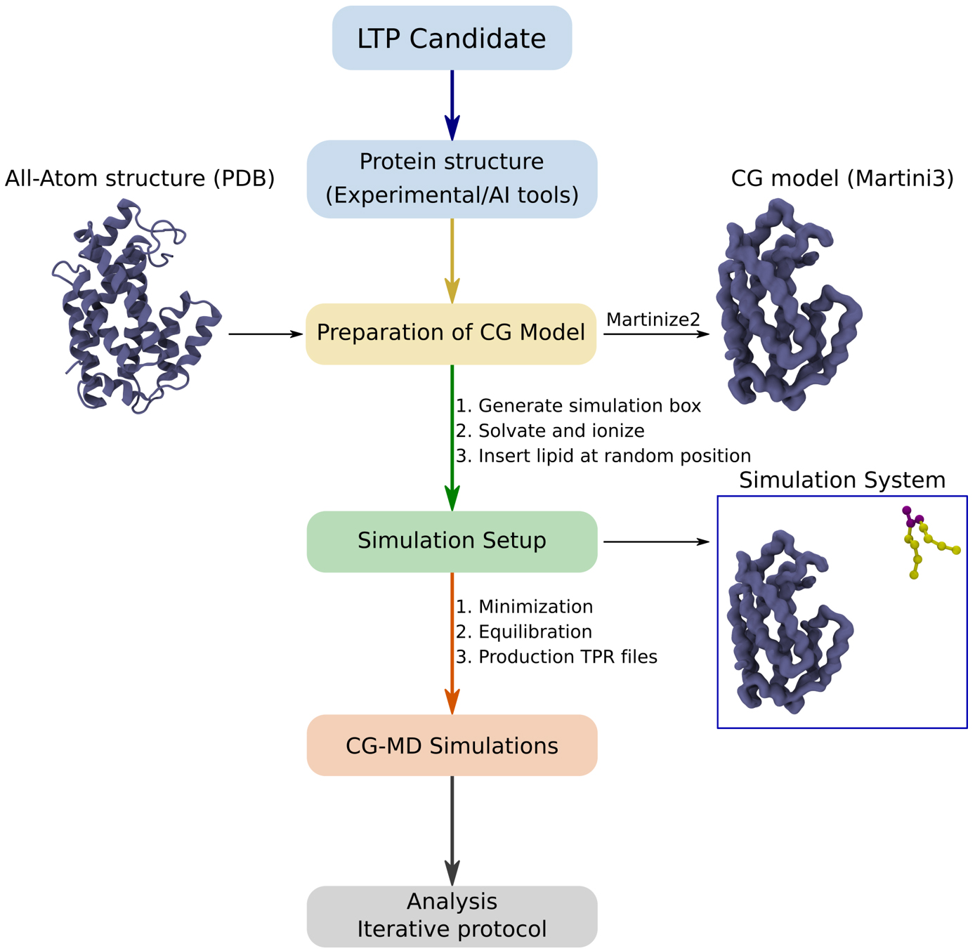
Figure 1. Different steps used in this protocol to identify lipid-binding cavities on a candidate lipid transfer protein (LTP)
A. Preparation of the CG model
Download the file workflow.sh as well as the common/ folder to your workstation using the following link: https://github.com/danialv4/Unbiased_simulations_characterize_lipid_binding/tree/main/Workflow/common.
Load the installed version of GROMACS on your workstation. Adjust the version number and GMXRC path if they differ from the example below. We have tested several versions of GROMACS for this protocol; any version newer than 2021.2 can be used to run it (e.g., the newest 2025.3), but older versions, although untested, may also work.
source /opt/GROMACS/2021.2/bin/GMXRCFor all proteins used in the publication corresponding to this manuscript, the CHARMM-GUI PDB Reader was used to generate the input all-atom structure. After unzipping the CHARMM-GUI output in the same folder that contains the workflow script, the file step1_pdbreader.pdb is used. However, any pre-processed protein structure is acceptable. If your file is called prepared_protein.pdb, replace all instances of step1_pdbreader in the subsequent four commands with prepared_protein.
Caution: The protocol can be run with AI-predicted structures, but we recommend checking the confidence in the prediction before running the protocol, as results with low-scoring predictions would not be meaningful.
Critical: If your protein has large, disordered regions, a possible cap at the binding cavity, or a small binding cavity, the protocol may require some modifications; see General notes 1, 2, and 3, respectively. In this sense, we have demonstrated that removing parts of the protein not located at the hydrophobic cavity, such as large, disordered loops, or the cap located at the entry of the binding cavity, can help with reproducing the experimental binding of lipids for LTPs. In addition, proteins with a tight hydrophobic cavity can be too restricted by a large force constant for the elastic network, so lowering it to 500 kJ·mol-1·nm-2 can add the flexibility to the protein structure necessary to reproduce lipid binding.
Once these steps are done, the script can be run directly from the folder ./workflow.sh. However, we explain below each of the commands and steps that the script contains:
cp ./charmm-gui*/step1_pdbreader.pdb step1_pdbreader_his.pdb #Copies file to current folderUpdate the naming of histidines and remove the hydrogen on ND (delta-nitrogen) to ensure proper recognition by the martinize2 script of unexpected errors.
sed -i ‘s/HSD/HIS/g’ step1_pdbreader_his.pdb #sed commands are used to change the text of a file without using a text editorsed -i ‘/HD1 HIS/d’ step1_pdbreader_his.pdbGenerate Martini topology (topol.top) and the coarse-grained structure of the protein (prot_cg_fc1000_eu8.pdb). The command used is shown below, followed by explanations of key options. Modify the path to DSSP, which is used to identify the secondary structure of the protein, as required. For additional details and available options, refer to the martinize2 documentation (https://vermouth-martinize.readthedocs.io/en/latest/martinize2_workflow.html) and the martinize GitHub repository (https://github.com/marrink-lab/vermouth-martinize).
martinize2 -f step1_pdbreader_his.pdb -x prot_cg_fc1000_eu8.pdb -o topol.top -ff martini3001 -elastic -ef 1000 -eu 0.8 -nt -scfix -cys auto -dssp /usr/bin/dssp-f: input all-atom PDB file to be coarse-grained
-x: output pdb file name
-o: output topology file name
-ff: force-field (here, we are using version 3001 of the protein model in Martini 3) [1]
-elastic: adds an elastic network to maintain the secondary structure of the protein
-ef: magnitude of the elastic force constant in kJ·mol-1·nm-2
-eu: upper cutoff for the elastic network
-nt: neutral termini for protein ends
-scfix: generalized side chain corrections
-cys: specify in case there are cysteine bonds
-dssp: path to the DSSP file on your system
-merge: (optional) merge chains and specify chain IDs for multimeric proteins.
Critical: Change the elastic network force constant (-ef) if your proteins would benefit from a more flexible structure, as explained above.
Place the coarse-grained protein in a cubic box with at least 2.0 nm between the solute and the edges using editconf in GROMACS.
Caution: We recommend not changing the 2 nm parameter, as shorter distances may hinder protein mobility, and artifacts from protein–protein interactions between PBC images may appear, and longer distances would increase the computational cost unnecessarily.
gmx editconf -f prot_cg_fc1000_eu8.pdb -c -d 2.0 -bt cubic -o prot_cg_newbox.groThe Martini 3 force-field (.itp) files used in the study, the initial coordinate (.gro) files for lipids and water, and the gromacs mdp parameters for minimization, equilibration, and production are provided in the common/ folder. Copy the CG topology file template into the working directory.
cp ./common/cg.top . #Copy the topology file to current folderB. Preparation of simulation setup
Perform an initial minimization of the coarse-grained protein in vacuum using the provided minimization parameters with GROMACS.
# Prepare the input binary (.tpr) for minimization in vacuumgmx grompp -f ./common/min-vac.mdp -p cg.top -c prot_cg_newbox.gro -o min-vac.tpr# Run the minimizationgmx mdrun -v -deffnm min-vacChoose which lipids to insert around the protein. Here, the example starts with DOPC, but you can uncomment and extend the array with other lipids (cholesterol, DPPC, TO, OLAC, DPSM, etc.). If you want to test the protocol with other lipids, just include a gro file with their coordinates to the common folder.
Caution: We recommend using DOPC lipids for a general test of whether the protein is able to bind lipids or not, as there is no general specificity for lipids using this protocol.
declare -a LipidArray=(“dopc”) #”chol” “dppc” “to” “olac” “dpsm”) #Array with all the testing lipidsFor each lipid type, the script generates five replicas to account for variability in random placement. First, for each replica, the lipid is inserted into the simulation box at a random position. Then, the system with the CG protein and lipid is solvated and ionized with NaCl 0.12 M, with additional ions to neutralize the net charge of the system. After that, the system is minimized and equilibrated, and TPR files for production are generated. These files can be used to run the production of each replica.
Caution: Five replicas of 1 ms each are normally enough to analyze lipid binding. However, larger LTPs, such as BLTPs, may require additional replicas and longer simulation times to reproduce binding in multiple replicas.
# Define the lipid(s) to testdeclare -a LipidArray=(“dopc”) # add “chol” “dppc” “to” “olac” “dpsm” as neededfor lipid in ${LipidArray[@]} #Loop for each of the lipidsdofor replica in `seq 1 5` #Loop for the 5 replicasdo######################### (a) Insert lipid molecules########################gmx insert-molecules -f min-vac.gro \-ci ./common/cg_${lipid}.gro \-nmol 1 \-o 1molecule_${lipid}_seed${replica}.gro######################### (b) Solvate with water########################gmx solvate -cp 1molecule_${lipid}_seed${replica}.gro \-cs ./common/water.gro \-radius 0.21 \-o solv_1molecule_${lipid}_seed${replica}.gro######################### (c) Update topology########################cp cg.top ${lipid}_seed${replica}.topecho “$lipid 1” | tr a-z A-Z >> ${lipid}_seed${replica}.top #Updated the topology file for each replicagrep -c W solv_1molecule_${lipid}_seed${replica}.gro | sed ‘s/^/W /’ >> ${lipid}_seed${replica}.top #This command counts the number of water molecules and includes this information in the topology file######################### (d) Pre-ionization setup########################gmx grompp -f ./common/ions-cg.mdp \-c solv_1molecule_${lipid}_seed${replica}.gro \-p ${lipid}_seed${replica}.top \-o ions_${lipid}_seed${replica}.tpr \-maxwarn 1######################### (e) Ionize with NaCl (0.12 M)########################echo 14 | gmx genion -s ions_${lipid}_seed${replica}.tpr \-o ions_${lipid}_seed${replica}.gro \-p ${lipid}_seed${replica}.top \-pname NA -nname CL \-neutral -conc 0.12######################### (f) Minimization of solvated & ionized system########################gmx grompp -f ./common/min-vac.mdp \-c ions_${lipid}_seed${replica}.gro \-p ${lipid}_seed${replica}.top \-o min-ions_${lipid}_seed${replica}.tprgmx mdrun -v -nt 4 -deffnm min-ions_${lipid}_seed${replica}######################### (g) Index file creation########################gmx make_ndx -f min-ions_${lipid}_seed${replica}.gro \-o index_${lipid}_seed${replica}.ndx < ./common/input_prot_nonprot.txt######################### (h) Equilibration (NPT ensemble)########################gmx grompp -f ./common/npt_eq.mdp \-c min-ions_${lipid}_seed${replica}.gro \-p ${lipid}_seed${replica}.top \-o npt_eq_${lipid}_seed${replica}.tpr \-n index_${lipid}_seed${replica}.ndx \-r min-ions_${lipid}_seed${replica}.grogmx mdrun -nt 4 -v -deffnm npt_eq_${lipid}_seed${replica}######################### (i) Generate production run TPR########################gmx grompp -f ./common/martini_v2.x_new-rf_3us.mdp \-c npt_eq_${lipid}_seed${replica}.gro \-t npt_eq_${lipid}_seed${replica}.cpt \-n index_${lipid}_seed${replica}.ndx \-p ${lipid}_seed${replica}.top \-o md_${lipid}_seed${replica}.tpr \-maxwarn 1 donedone The production TPR files can be executed either locally on your workstation or submitted to a high-performance computing (HPC) cluster. The replicas can be run sequentially (one after another) with the command option A or launched in parallel, if resources allow, by running command B for each replica, replacing ${lipid} with the lipid name and ${replica} with the replica number.
# Option Afor lipid in ${LipidArray[@]}dofor replica in `seq 1 5`dogmx mdrun -nt 4 -v -deffnm md_${lipid}_seed${replica}donedone# Option Bgmx mdrun -nt 4 -v -deffnm md_${lipid}_seed${replica}C. Visualization and analysis of the results
The scripts for all analyses performed in the associated publication are available on GitHub at https://github.com/danialv4/Unbiased_simulations_characterize_lipid_binding/tree/main/Analysis. In this section, we focus on the analysis of lipid tail solvation, which served as the key metric for distinguishing lipid-binding events to cavities in LTPs from those where lipids either remained in water or adhered to the external surfaces of the protein. This analysis counts, for each frame, the number of water molecules within 0.5 nm of the lipid tails. This short cutoff allows counting the water molecules closer to the lipid tails without adding noise from the solvent bulk molecules. We recommend not changing this parameter, regardless of the lipid type.
When running the code, you will be prompted to include the name of the lipid you are using. This will only affect the file names that are read and written.
#Select the lipid for which to compute the solvation interactivelyecho “lipid?”read lipidThen, the five replicas of the corresponding lipid are analyzed using the same script. The analysis script runs in VMD and is readily generated (calc_$lipid$val.vmd) and deleted after use. The file named “calc_$lipid$val.txt,” which is also generated in the script, runs the analysis and closes VMD after finishing it. Make sure to change the lipid tail bead names to the ones of the lipid you are analyzing. In the example below, for a DOPC lipid, the names are “C1A D2A C3A C4A C1B D2B C3B C4B.” The results of the individual replicas are written in separate files named “water_around_lipid_$lipid_seed$val_time.dat,” which include the frame numbers as well as the lipid tail solvation per frame.
Critical: Please select the bead names for the lipid tails that correspond to the tested lipid. These names can be directly inferred from the topology or the structure of the coarse-grained lipid. We recommend visualizing it with VMD and selecting all the beads that form the lipid tails.
for val in `seq 1 5`docat >source_$lipid$val.txt << EOFsource calc_$lipid$val.vmdexitEOF#Make sure to change the lipid tail beads according to your simulated lipidcat >calc_$lipid$val.vmd << EOFmol delete allmol new ./md_${lipid}_seed${val}_prot_center_pbcmol.gromol addfile ./md_${lipid}_seed${val}_prot_center_pbcmol.xtc waitfor allset file [open “water_around_lipid_${lipid}_seed${val}_time.dat” w]set sel [atomselect top “name W and pbwithin 5 of (name C1A D2A C3A C4A C1B D2B C3B C4B)”]set n [molinfo top get numframes]for {set i 0} {$i<$n} {incr i} {$sel frame $i$sel updateset len1 [llength [lsort -unique [$sel get resid]]]puts $file “$i $len1”}close $fileexitEOF vmd -dispdev none -e source_${lipid}${val}.txtdonerm calc_$lipid*vmdrm source_$lipid*txtThe results can either be visualized as time traces, which will show a depletion of the solvation of the lipid tails once the binding occurs, or used to make boxplots/violinplots, which will display a lower solvation for the replicas with lipid binding with respect to the ones without binding. Binding is therefore confirmed when the lipid is bound to the cavity of the tested protein and presents low solvation numbers for the lipid tails. For examples and representative values for positive and negative controls, see [2]. In general, lipid tail solvation numbers of less than 2 are indicative of lipid binding to a hydrophobic cavity.
D. Iterative protocol for LTPs that can bind multiple lipids
To examine how lipids occupy bridge-like LTPs (BLTPs) or LTPs with large binding cavities that may accommodate multiple lipids at the same time, like synaptotagmin-like mitochondrial-lipid-binding (SMP) proteins, we adapted our simulation workflow to perform an iterative lipid addition process. Lipid molecules are introduced step by step, rather than all at once, to minimize premature lipid–lipid interactions in solution that could otherwise lead to micelle formation before binding to the protein. At each iteration, the final frame of the trajectory containing n bound lipids is saved and used as the input for introducing the (n+1)th lipid.
For instance, after one lipid has successfully bound to the LTP, the protein–lipid coordinates (with no solvent and ions) from the last trajectory frame must be saved as a separate GRO file, and the workflow is repeated. This means that the second round begins with one lipid in the cavity and one in the solvent, while the third round begins with two lipids in the cavity and one in the solvent, and so forth. The system is re-solvated and re-ionized at each round of iteration.
This iterative process continues until no additional lipids enter the hydrophobic cavity.
To modify the workflow.sh script for multiple lipid binding, please find the script change.sh in https://github.com/danialv4/Unbiased_simulations_characterize_lipid_binding/tree/main/Workflow. You will first be prompted to specify the number of simultaneous lipids you want to test (n+1) and then the GRO file with n lipids bound, which must be in the same folder. The script generates a workflow $(n+1) sh script that is ready to use. The name of the new files will end with $(n+1) to distinguish them from the original ones.
echo “Total number of lipids to test”read nlecho “GRO file with n number of bound lipids”read initialsed 1,17d workflow.sh > workflow$nl.shsed -i 5,8d workflow$nl.shsed -i “s/prot_cg_fc1000_eu8.pdb/$initial/g” workflow$nl.shsed -i “s/prot_cg_newbox/prot${nl}_cg_newbox/g” workflow$nl.shsed -i “s/min-vac.gro/prot${nl}_cg_newbox/g” workflow$nl.shsed -i “s/\${replica}/\${replica}_$nl/g” workflow$nl.shsed -i “s/\$lipid 1/\$lipid $nl/g” workflow$nl.shValidation of protocol
This protocol has been used and validated in [2], using LTPs with X-ray structures that contained lipid ligands as well as negative controls. In this sense, we have compared the binding poses of lipids to experimental X-ray structures and tested point mutations of BLTPs that had been tested experimentally. On the other hand, as negative controls, we have tested the protocol against proteins with large hydrophilic cavities, showing no false positives.
General notes and troubleshooting
General notes
1. For proteins with large intrinsically disordered regions (IDR), we recommend not including these regions, whenever possible, as they are normally not part of the lipid-binding domain and may hinder lipid binding.
2. One drawback of CG-MD simulations is the lack of conformational changes. This can lead to technical problems if the lipid-binding domain presents a cap that may open and close to allow lipid binding/release, as this conformational change will not be observed in CG-MD simulations. For those cases, we recommend deleting the cap, so the entry to the hydrophobic cavity is always open. For example, the cap present in Osh proteins (such as Osh4 and Osh6) hinders lipid binding unless it is removed from the structure.
3. The structure of some proteins may be in the apo form, with the cavity too small for the tested lipids. In those cases, using a lower force constant (e.g., 300 kJ·mol-1·nm-2) or a lower distance cutoff for the elastic network may help. For instance, when testing StARD11, and due to the tightness of its hydrophobic cavity, lipid binding could only be observed after lowering the force constant to 300 kJ·mol-1·nm-2.
4. The protocol can return false negatives in multiple replicas, showing no lipid binding even for LTPs. This problem can be attenuated by increasing the production simulation time to 3 ms or by running more replicas.
Troubleshooting
Problem 1: Martinize2 problem due to the DSSP version, lack of compatibility with new versions of DSSP.
Possible cause: Use of newer DSSP versions.
Solution: Try to install an older version (like 3.0.0) whenever possible. Alternatively, you can remove the path to your DSSP in the martinize2 command, and mdtraj will be used instead to predict the secondary structure of the protein.
Problem 2: Lack of protein–lipid interactions in many replicas.
Possible cause: The protein is too large, so the simulation box is too big.
Solution: Increase the production simulation time to 3 ms. The MDP file is provided in the common folder.
Acknowledgments
Contributions: Conceptualization, D.A., S.V., S.S.; Investigation, D.A., S.V., S.S.; Writing—Original Draft, D.A., S.S.; Writing—Review & Editing, D.A., S.V., S.S.; Funding acquisition, S.V.
S.V. acknowledges support from the Swiss National Science Foundation (grants ID CR00I5-236020) and by the European Research Council under the European Union’s Horizon 2020 research and innovation program (grant agreement no. 803952). This work was supported by grants from the Swiss National Supercomputing Centre under projects ID s1269, lp24, and lp69. The protocol described in this paper was originally published in [2], which was based on [8].
Competing interests
The authors declare no conflicts of interest.
References
- Souza, P. C. T., Alessandri, R., Barnoud, J., Thallmair, S., Faustino, I., Grünewald, F., Patmanidis, I., Abdizadeh, H., Bruininks, B. M. H., Wassenaar, T. A., et al. (2021). Martini 3: a general purpose force field for coarse-grained molecular dynamics. Nat Methods. 18(4): 382–388. https://doi.org/10.1038/s41592-021-01098-3
- Srinivasan, S., Álvarez, D., John Peter, A. T. and Vanni, S. (2024). Unbiased MD simulations identify lipid binding sites in lipid transfer proteins. J Cell Biol. 223(11): e202312055. https://doi.org/10.1083/jcb.202312055
- Kroon, P. C., Grunewald, F., Barnoud, J., van Tilburg, M., Brasnett, C., de Souza, P. C. T., Wassenaar, T. A. and Marrink, S. J. (2025). Martinize2 and Vermouth: Unified Framework for Topology Generation. eLife. 12: e3. https://doi.org/10.7554/elife.90627.3
- Kabsch, W. and Sander, C. (1983). Dictionary of protein secondary structure: Pattern recognition of hydrogen‐bonded and geometrical features. Biopolymers. 22(12): 2577–2637. https://doi.org/10.1002/bip.360221211
- Abraham, M. J., Murtola, T., Schulz, R., Páll, S., Smith, J. C., Hess, B. and Lindahl, E. (2015). GROMACS: High performance molecular simulations through multi-level parallelism from laptops to supercomputers. SoftwareX. 1–2: 19–25. https://doi.org/10.1016/j.softx.2015.06.001
- Humphrey, W., Dalke, A. and Schulten, K. (1996). VMD: Visual molecular dynamics. J Mol Graphics. 14(1): 33–38. https://doi.org/10.1016/0263-7855(96)00018-5
- Jumper, J., Evans, R., Pritzel, A., Green, T., Figurnov, M., Ronneberger, O., Tunyasuvunakool, K., Bates, R., Žídek, A., Potapenko, A., et al. (2021). Highly accurate protein structure prediction with AlphaFold. Nature. 596(7873): 583–589. https://doi.org/10.1038/s41586-021-03819-2
- Souza, P. C. T., Thallmair, S., Conflitti, P., Ramírez-Palacios, C., Alessandri, R., Raniolo, S., Limongelli, V. and Marrink, S. J. (2020). Protein–ligand binding with the coarse-grained Martini model. Nat Commun. 11(1): 3714. https://doi.org/10.1038/s41467-020-17437-5
Article Information
Publication history
Received: Oct 3, 2025
Accepted: Nov 16, 2025
Available online: Dec 9, 2025
Published: Dec 20, 2025
Copyright
© 2025 The Author(s); This is an open access article under the CC BY-NC license (https://creativecommons.org/licenses/by-nc/4.0/).
How to cite
Readers should cite both the Bio-protocol article and the original research article where this protocol was used:
- Álvarez, D., Vanni, S. and Srinivasan, S. (2025). Identifying and Characterizing Lipid-Binding Cavities in Lipid Transfer Proteins With CG-MD Simulations. Bio-protocol 15(24): e5558. DOI: 10.21769/BioProtoc.5558.
- Srinivasan, S., Álvarez, D., John Peter, A. T. and Vanni, S. (2024). Unbiased MD simulations identify lipid binding sites in lipid transfer proteins. J Cell Biol. 223(11): e202312055. https://doi.org/10.1083/jcb.202312055
Category
Bioinformatics and Computational Biology
Biophysics > Macromolecular simulations
Do you have any questions about this protocol?
Post your question to gather feedback from the community. We will also invite the authors of this article to respond.