- Protocols

- Articles and Issues
- For Authors
- About
- Become a Reviewer

Using Beads as a Focus Fiduciary to Aid Software-Based Autofocus Accuracy in Microscopy
Published: Vol 15, Iss 14, Jul 20, 2025 DOI: 10.21769/BioProtoc.5388 Views: 1135
Reviewed by: Anonymous reviewer(s)
Advertisement


Protocol Collections
Comprehensive collections of detailed, peer-reviewed protocols focusing on specific topics


Abstract
Brightfield microscopy is an ideal application for studying live cell systems in a minimally invasive manner. This is advantageous in long-term experiments to study dynamic cellular processes such as stress response. Depending on the sample type and preparation, the inherent qualities of brightfield microscopy, being very low contrast, can contribute to technical issues such as focal drift, sequencing lags, and complete failure of software autofocus systems. Here, we describe the use of microbeads as a focus aid for long-term live cell imaging to address these autofocus issues. This protocol is inexpensive to implement, without extensive additional sample preparation, and can be used to capture focused images of transparent cells in a label-free manner. To validate this protocol, a widefield inverted microscope was used with software-based autofocus to image overnight in time-lapse format, demonstrating the use of the beads to prevent focal drift in long-term experiments. This improves autofocus accuracy on relatively inexpensive microscopes without using hardware-based focus aids. To validate this protocol, the KNIME logistics software was used to train a random forest model to perform binary image classification.
Key features
• Label-free live cell imaging in time-lapse format.
• Troubleshooting software autofocus for brightfield mode.
Keywords: Live-cell imagingGraphical overview
Background
In fluorescence microscopy, fluorescent stains and probes can be used to highlight subcellular structures. The caveats of using fluorescent microscopy, such as photobleaching and phototoxicity, are well described [1]. Phototoxicity refers to the process where typical wavelengths that are used in fluorescence imaging generate excessive reactive oxygen species (ROS), which can lead to DNA damage [2]. This phenomenon is dependent on wavelength and length of exposure to cells [2]. Intracellular ROS production can be buffered by cell antioxidant molecules and enzymes, although in fluorescent imaging, ROS buffering capacities can be exceeded [3,4]. Photobleaching refers to the destruction of a fluorophore, such as a fluorescent protein (i.e., GFP), in the excited state that leads to depletion of signal over time; this can result in the production of ROS and subsequent photobleaching [1,5].
Commonly used stains such as DRAQ5 and Hoechst that highlight chromatin have demonstrated cytotoxic effects in live-cell imaging [6,7]. DRAQ5 dye alters the dynamics and localization of critical proteins involved in DNA transcription, replication, and repair; Hoechst can cause cell cycle arrest or delay of the G2 phase [6,7]. Consideration must be taken when designing experiments to minimize the confounding effects of potentially cytotoxic stains (phototoxicity and photobleaching), especially in long-term acquisitions. This is necessary as artifacts may appear from sample preparation and/or in imaging, and this becomes increasingly important when evaluating the effects of cell treatments.
Time-lapse experiments are easily susceptible to phototoxicity. Cell migration is reduced at high fluorescent light doses compared with cells imaged in brightfield [8]. Time resolution and/or light dose must be compromised to reduce phototoxicity using fluorescent microscopy, making this unsuitable to follow rapid cellular activities [9]. In contrast, brightfield microscopy is label-free, making this technique less invasive and relatively inexpensive. This is an ideal application for studying live-cell systems and processes that are sensitive to oxidative stress caused by elevated ROS, such as mitosis [4,10]. Additionally, information that may differ from fluorescent images, such as cell texture, can be acquired simultaneously with structural information to create novel morphological profiles [11].
Autofocus combines search algorithms and focus metrics to identify the sharpest image across the entire focal depth [12,13]. In automated microscopy, focus metrics are contrast-based algorithms applied to each image when scanning the focal depth. Plotting the magnitude of the focus function creates a focal curve where the most focused image is the global maximum [12]. Ideally, the range of the focus curve is narrow, creating a single defined global maximum with few, if any, local maxima [10]. In practice, when evaluated across different sample types, commonly used focus metrics are far from robust, and the focal curve is not unimodal [14–16].
Confounding the susceptibility of focus metrics to failure, search algorithms are another possible source of error in autofocus. These algorithms represent optimization problems, where the most focused image must be defined accurately and rapidly. Global search is a commonly used search algorithm that samples the entire focal depth but is computationally slow. To optimize speed, the hill climbing method is a type of binary search using a combination of fine and rough focusing; however, it can incorrectly select a local maximum as the most focused image [16]. The susceptibility to failure of autofocus systems appears frequently in the presence of plate scratches, debris, noise, lack of high-frequency content (i.e., few cells, transparent cells), or uneven illumination [14,15]. High-frequency content is associated with sharp objects. Contrast-based autofocus systems identify the global maximum by comparing sharpness across the focal depth [14].
Autofocus algorithms have been evaluated and implemented effectively with fluorescence microscopy, due to the inherent high signal-to-noise ratio [17]. Despite mitigating many drawbacks associated with fluorescence microscopy, the qualities of brightfield microscopy make it more susceptible to autofocus problems. For example, imaging transparent cells such as fibroblasts produces images with low signal-to-noise ratios and makes identifying the correct focal plane by autofocus more error-prone.
Our goal was to utilize an inverted widefield microscope with software autofocus to capture mitotic events in hTERT immortalized patient-derived fibroblasts, also known as TruHD cells [18], to study the impact of Huntington’s disease-associated mutations on cell growth. Since increased cell stress and sensitivity to DNA damage have been demonstrated in TruHD cells [18], we wished to mitigate additional cell stress by choosing to collect brightfield stain-free images. However, we found the software-based autofocus insufficient for use in the transmitted light channel specifically (Figure 1). This failure could not be resolved by imaging in phase contrast or by selecting an alternative built-in autofocus algorithm. In collecting temporal data over time without the aid of autofocus, we observed drift from the manually set focus over time, even while using stains, demonstrating that a working autofocus is necessary to acquire quality movies. In this paper, we describe in detail the use of microbeads as an aid for focusing on the transmitted light channel to acquire images of live cells in time-lapse.
This method is not only effective in eliminating long-term focus drift; in multi-well plates, placing beads in wells adjacent to wells without beads aids focus accuracy. In place of tedious manual annotation of over 3,700 images collected using this protocol, a random forest model was trained. The model was used to perform unbiased binary classification, identifying images as focused or unfocused. The classifier is not required to use beads as a focal fiduciary; however, this was essential to validate this method. This protocol will briefly describe training the machine learning algorithm using the data analysis platform, KoNstanz Information MinEr, or KNIME ( https://www.knime.com/).
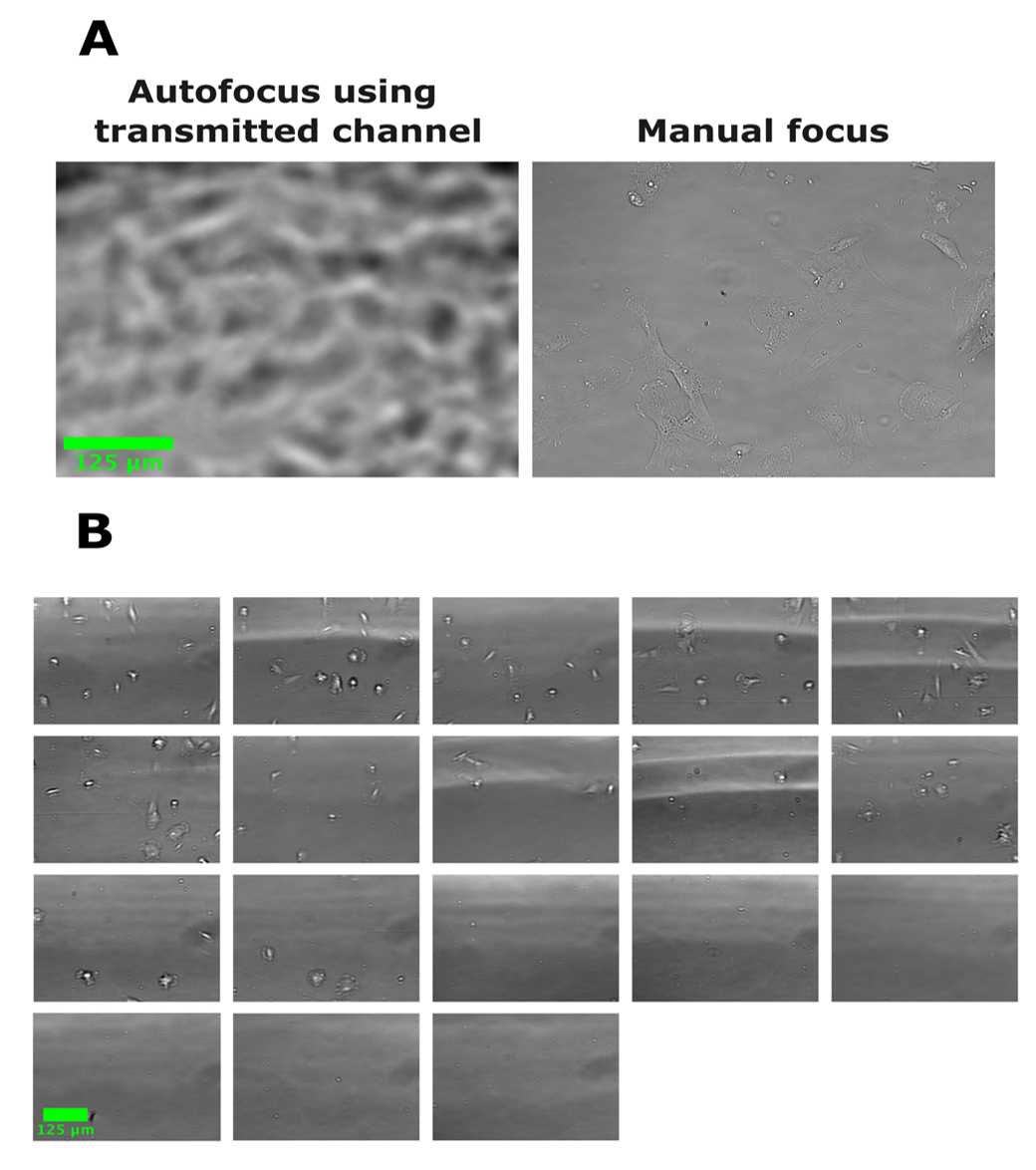
Figure 1. Software autofocus can fail when acquiring brightfield images. In all images, human fibroblasts were seeded in a 384-well plate and images were acquired with a 20× objective Plan fluorite (Evos, NA = 0.5). (A) Example brightfield image acquired using autofocus compared with an image focused manually. Autofocus fails to find the correct plane of focus based on the transmitted light channel. (B) Images acquired of other wells of the same plate from (A) in a single automated scan using autofocus. All images show the failure of autofocus using the transmitted channel to focus.
Materials and reagents
Biological materials
1. TruHD Cells [16]
Reagents
1. Minimal essential media (MEM), 1× (Gibco, catalog number: 10370-021)
2. Fetal bovine serum (Wisent, catalog number: 098450)
3. Deionized microfiltered water
Solutions
1. Supplemented media (see recipes)
Recipes
1. Supplemented media
| Reagent | Final concentration | Quantity or volume |
|---|---|---|
| MEM 1× | n/a | 500 mL |
| Fetal bovine serum | 13% | 75 mL |
| Total | n/a | 575 mL |
Laboratory supplies
1. 0.2 μm filter (Filtropur BT50, 83.3941.101)
2. 50 mL Screw cap tube (Starstedt, 62.547.254)
3. Microbeads: Silicon dioxide microparticles 2 μm (Sigma-Aldrich, catalog number: 81108-5ML-F), red fluorescent latex beads 2 μm (Sigma-Aldrich, catalog number: L3030-1ML), and non-fluorescent latex beads 3 μm (Sigma-Aldrich, catalog number: LB30-2ML)
Note: Beads are stored at room temperature and covered in foil.
4. 384-well plate (PerkinElmer, PhenoPlate)
5. Hemocytometer (any)
6. “Dummy” plate (any)
7. Pipette tips: 10 μL (VWR, catalog number: 76322-528), 200 μL (VWR, catalog number: 76322-150), and 1000 μL (VWR, catalog number: 76322-154)
8. Pipette: p10 (Eppendorf, catalog number: 3123000020), p200 (Eppendorf, catalog number: 3123000055), and p1000 (Eppendorf, catalog number: 3124000121
9. 1.5 mL microcentrifuge tubes (Avantar, catalog number: 20170-038)
10. Tissue culture plates (Fisherbrand, catalog number: FB012924)
11. Microtube rack (Any)
Equipment
1. Multi-gas incubator (PHCBI, catalog number: MCO-170M-PA)
2. Evos M7000 microscope (ThermoFisher, catalog number: AMF7000)
a. EVOS onstage incubator (Invitrogen, catalog number: AMC1000)
b. EVOS objective lens (20× Air, Plan fluorite 20×/NA 0.5, catalog number: AMEP4698)
c. EVOS light cube (Cy5, catalog number: AMEP4956)
3. Laboratory plate centrifuge (Eppendorf, model: Centrifuge 5810R)
4. Biological safety cabinet (Microzone corporation, model: BK-2-4)
Software and datasets
1. Python (3.10.9)
2. EVOS imaging software (2.1.677.717)
3. GraphPad Prism (10.2.3)
4. KNIME (5.2.1)
5. System requirements:
a. Linux: 64-bit, at least 8 GB RAM
b. Mac: 10.11 and above, at least 8 GB RAM
c. Windows: 32- or 64-bit, at least 8 GB RAM
Procedure
A. Day 1: Plate preparation
See General note 1.
Critical: This protocol describes Experiment 2 (Figure 2); 2 μm red latex beads are used.
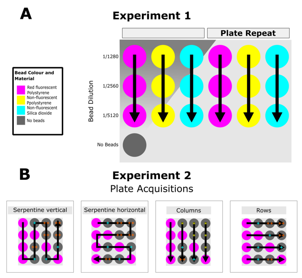
Figure 2. Graphical schematic of the experimental protocol used for validation. Images analyzed were acquired using two different experimental protocols set up on an EVOS M7000. In both A and B, black arrows indicate the directionality of the selected scan protocol, and the color of the well indicates well content (see legend in A). For further details of the autofocus procedure used, see the data acquisition section. (A) Experiment 1 was used to evaluate the efficacy of different bead materials and fluorescence using polystyrene (PS) 2 μm, PS 3 μm, and silica dioxide (glass) 2 μm. (B) Experiment 2 was designed to determine whether the presence of beads in the well, or in a neighboring well, reduces imaging lags and focus drift. Red fluorescent beads (2 μm) were used. The transmitted channel was selected as the focus channel and the single channel acquired. The same sample was imaged in quadruplicate using four different scanning routings: serpentine vertical, serpentine horizontal, column-wise, and row-wise. Wells marked with a yellow asterisk highlight wells where images were acquired before a well containing microbeads; a blue plus sign highlights wells that were imaged directly following (adjacent) a well containing microbeads; two orange plus signs highlight wells that were imaged within two or more wells following a well containing microbeads. Plate metadata was extracted from all four plate scans, providing the time each image was acquired. The exposure time per well was determined as the time between the first and last frame taken in each well. Subsequently, data were sorted based on the presence or absence of beads in the well images. Wells that did not contain beads were further sorted into three categories based on the order imaged (before or after imaging beads) and their relative position in the plate (1 or 2+ wells away from a well with beads).
1. Cell counting
a. Add 300 μL of suspended cells to a screw cap tube.
b. Add 3 mL of supplemented media to the tube.
c. Mix thoroughly.
d. Add a small volume of the mixture (5 μL) to a hemocytometer.
e. Follow the directions provided for the hemocytometer to determine cell dilution.
f. Dilute the cells to 15 cells/μL using supplemented media.
2. Seed 384-well plate
a. Add 50 μL of the diluted cells from step A1 to each well as shown in Experiment 2 (Figure 2).
b. Leave the plate at room temperature for 15 min to allow cells to settle on the bottom of the well.
c. Place the plate into the incubator overnight (37.0 °C, 5.0% CO2, 8.0% O2).
B. Day 2: Bead dilution in filtered water
Critical: Cells should be 40%–50% confluent.
See General note 2 and 3.
1. Filter deionized water using a 0.2 μm filter.
2. Label microcentrifuge tubes.
a. Place six microcentrifuge tubes into the microtube rack.
b. Label with dilutions as follows: 1/11, 1/352, 1/704, 1/1408.
3. Add filtered water to the tubes as follows:
a. Add 50 μL of water to 1/11.
b. Add 155 μL of water to 1/352.
c. Add 100 μL of water to all remaining tubes (from step A2).
4. Serially dilute beads
a. Add 5 μL of beads to the 1/11 tube.
b. Mix thoroughly by pipetting at least 10 times.
c. Add 5 μL of the 1/11 to the 1/352 tube.
d. Mix thoroughly by pipetting at least 10 times.
e. Add 100 μL of the 1/352 dilution to the 1/704 tube.
f. Mix thoroughly by pipetting at least 10 times.
g. Add 100 μL of the 1/704 dilution to the 1/1408 tube.
C. Day 2: Addition of beads to the pre-seeded 384-well plate
1. Dilute the beads in media
a. Label a new microcentrifuge tube as 1/1408M.
b. Add 200 μL of supplemented media to the 1/1408M tube.
c. Add 25 μL of the beads from the 1/1408 dilution to the 1/1408M.
d. Aliquot 275 μL of supplemented media to a new microcentrifuge tube (25 μL per well is the minimum volume).
2. Add the beads to the plate (see General note 4)
a. From the 1/1408M, add 25 μL of the beads to bead wells as shown in Experiment 2 (Figure 2) to achieve a final dilution of 1/38,016.
b. Add 25 μL of aliquoted media to wells without beads as shown in Experiment 2 (Figure 2).
3. Spin down the plate at 1,000× g for 5 min.
Critical: Carefully remove the plate from the centrifuge, avoiding tilting and sudden movements. Disrupting the beads after spinning the plate will cause them to resuspend in the media. Avoid any sudden movements when transferring the plate to the microscope and handling it after this step.
D. Day 2: Collecting image data
1. Start the EVOS M7000 system.
2. Insert a “dummy” plate onto the stage to fill the space while the microscope is warming up.
3. Fill the incubator system with water.
4. Open the CO2 tank for delivery to the sample.
5. In the EVOS software, manually activate the environmental controls (5% CO2, 37 °C).
6. Allow the system to warm up for 1 h before use.
7. Transfer the plate to the microscope.
a. Data acquisition:
i. Experiment 1 (Figure 2) (see General note 5 and 6)
1) Imaging frequency and protocol: Serpentine vertical scanning, single passage of the plate, and 4 fields per well.
2) Autofocus settings: Algorithm selected: fluorescence optimized, autofocus with all channels, every field, first time point only, skip fields that fail.
3) Objective/channels acquired: 20× Plan fluorite, Transmitted, and Cy5.
ii. Overnight scanning procedure (Experiment 2, Figure 2):
1) Imaging frequency and protocol: Serpentine vertical scanning, acquire plate every 4 min for 14 h, and 4 fields per well.
2) Autofocus setting: Algorithm selected: fluorescence optimized, autofocus every field using transmitted channel, every time point, without skipping fields that fail.
3) Objective/channel acquired: 20× Plan fluorite, Transmitted.
Data analysis
Validation of this protocol was carried out with three technical replicates and two biological replicates. The training of the random forest model is briefly described below to validate this protocol. The model is unnecessary to implement beads as a focal fiduciary.
A. Image metadata analysis
Two scripts were created to extract metadata from the images acquired and used to create a CSV file containing the exposure time in each well. Next, this was sorted based on the position of the well. All scripts used for data analysis can be found on the Truant Lab GitHub at https://github.com/TruantLab/Py-files-Bio-Protocols- .
B. Sample time-lapse video creation
Images were selected from Experiment 2 (Figure 2) of a well with beads and an adjacent well (1st adjacent). The images were scaled using the mean pixel intensity of each image set, with a Python script also found on the Truant Lab GitHub.
C. Image classification in KNIME
The workflow described in this protocol is available at https://hub.knime.com/s/fbbMd4SW0FRbecm4.
D. Training a random forest model in KNIME
D1. Data preparation and feature extraction in CellProfiler
374 brightfield images were selected to generate a training dataset. Images were manually annotated with the ground truth class (focused, not focused). In CellProfiler, each image was filtered using either a Gaussian filter and/or an edge detection filter. From each image, texture features were extracted from the raw image or filtered images and exported to a database file. Features were graphed to identify candidates to train the image classifier in KNIME. Identified features demonstrated some ability to distinguish between image classes (i.e., focused, not focused) annotated earlier. The features selected include angular second moment (extracted from raw images), contrast and sum average (extracted from Gaussian-filtered images), and contrast (extracted from images with Gaussian and edge-detection filters applied). Features were extracted with a filter size of 170 pixels. A test set and all deployment data (i.e., images generated from repeats of this protocol) were analyzed through the CellProfiler pipeline, and features were extracted to separate database files.
D2. Design of a random forest model training architecture in KNIME
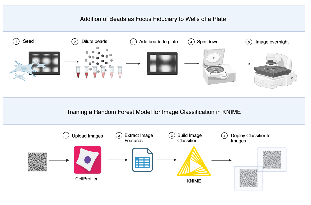
The KNIME workflow consists of training data pre-processing and annotation, training, validation, hyperparameter optimization, and deployment (Figure 3).
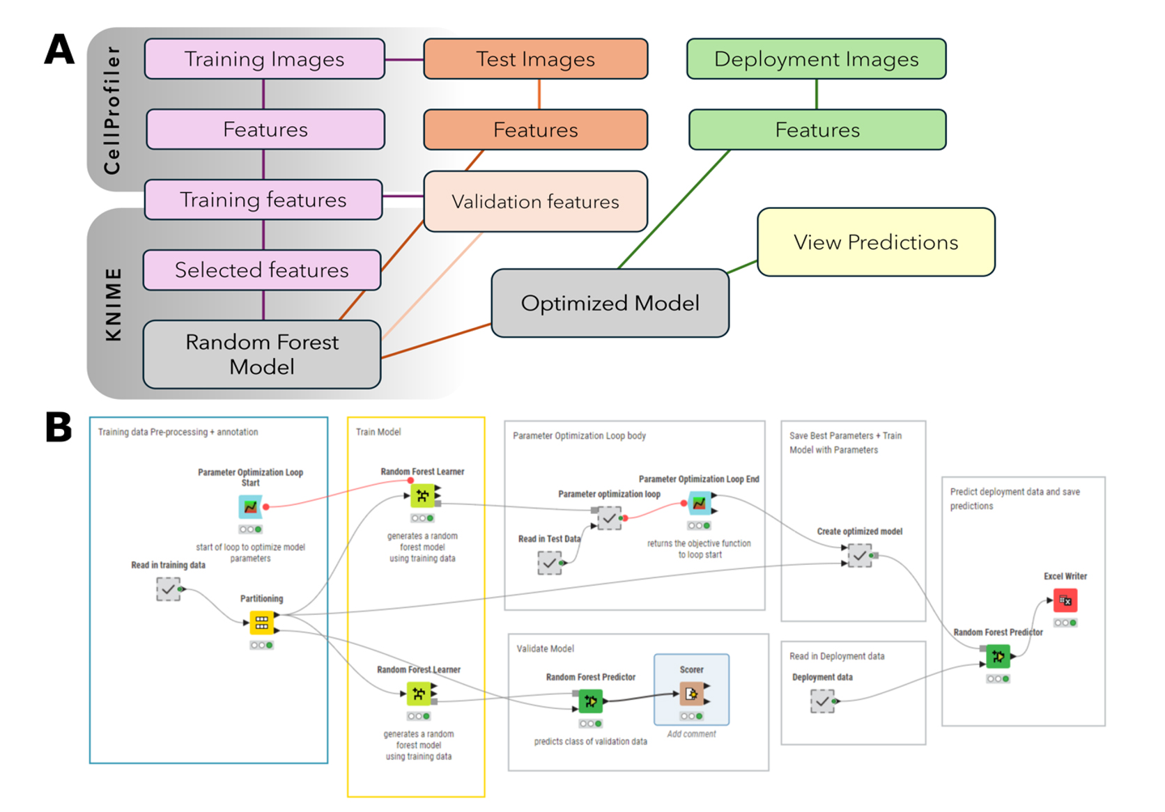
Figure 3. Overview of training a random forest image classifier in KNIME. (A) In CellProfiler, image features are extracted from the training, test, and deployment images. The features selected for training are read into KNIME and used to train a random forest model to classify images as focused or unfocused. Test features are used to optimize the model. Image features from the deployment images are read into the workflow and classified using the optimized model. (B) Image of KNIME workflow used to train a random forest model. The workflow consists of pre-processing, validation, hyperparameter optimization, and deployment. Pre-annotated training data is read into the workflow. Features selected for training are extracted, and a second annotation of this data is performed to generate a class variable in KNIME. Training features are divided between validation and training. A loop is used for hyperparameter optimization to determine an appropriate number of models and tree depth to use. The same features selected for training are extracted from the test data and used along with the training data for model optimization. The test set is used to generate the objective value, which indicates the performance of each set of hyperparameters as they are evaluated. The best-performing hyperparameters are saved to a table and used to train the deployment model. As before, the same features selected for training are extracted from the deployment data. The classifier is applied to these features, and predictions are exported to a spreadsheet file (MS Excel).
D3. Probability of a focused image
Images acquired in Experiment 2 (Figure 2) were predicted using the KNIME classifier. The probability of a focused image was calculated as the ratio of focused images to total images acquired in each field.
D4. Model validation, optimization, and test data
The model performed with 98.23% accuracy with a validation set of the training data. The model had 75% accuracy with the test set before optimization. Following optimization, the model’s accuracy improved to 92.97% with the test set.
Validation of protocol
To evaluate the use of this protocol, two criteria were selected: the presence of imaging lags and the ability to retain focus in overnight image acquisitions, as shown by Experiment 2 in Figure 2. The utility of microbeads other than that used for the overnight experiments was evaluated as shown in Experiment 1 (Figure 2). The effect of adding beads to a well was determined by compiling images in time-lapse format. The image classifier was used to evaluate the effect of the beads on adjacent wells.
1. Assessing the consistency in exposure time per well in the presence and absence of beads
Experiment 2 was designed to determine whether the presence of beads in the well or in a neighboring well reduces imaging lags. In preliminary experiments, we noticed imaging lags within the first passage of the plate, whereby the autofocus feature would expose certain wells longer than others.
The addition of the microbeads promoted consistent exposure time for wells with beads and significantly decreased mean acquisition time as compared to wells before beads (Figure 4). This indicates that the presence of the beads reduced and maintained consistent exposure time across multiple wells. We did not observe a difference in exposure time in wells adjacent to the beads compared to wells before the beads. This demonstrates that there is no improvement in the exposure time in adjacent wells. Therefore, having beads in the wells imaged is necessary for consistently low exposure time. However, changes to exposure time per well are not necessarily predictive of image focus. To assess this, we determined a means of classifying image focus to further validate the use of this protocol.
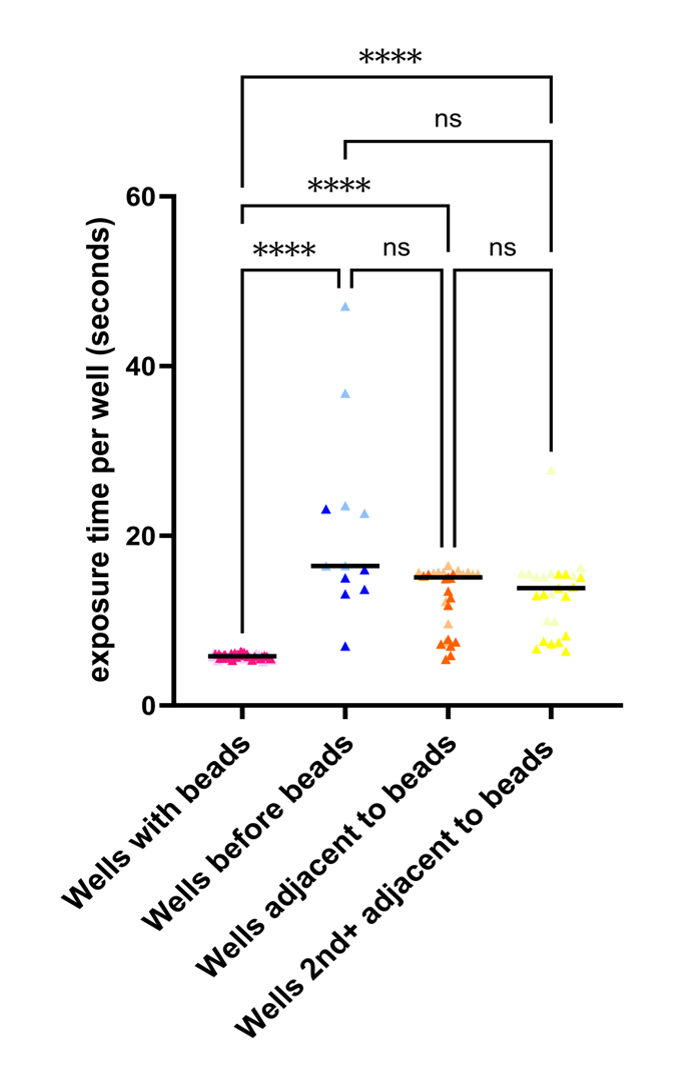
Figure 4. The presence of microbeads in a well reduces exposure time and does not extend to adjacent wells. Images were acquired as described in Experiment 2 (see Figure 2B). All analysis, excluding graphing, was completed in Python. Metadata was extracted from all four plate acquisitions as illustrated in Figure 2B, and the exposure time per well was calculated as the time point difference between the first and last images acquired in each well. Data was separated into i) wells with beads, ii) wells before beads, iii) wells adjacent to beads, and iv) wells 2nd+ adjacent to beads. Images acquired of the same well were included in the same or different data sets (i.e., wells with beads) if these came from different plate scans. Kruskal–Wallis Test was performed in GraphPad Prism (10.2.3). ***, P < 0.0001; ns, P > 0.05; n = 2.
2. Long-term acquisition image quality
Following four plate acquisitions, the plate was imaged in serpentine vertical for 14 h (Figure 2). In the time-lapse movies created from the images, the presence of the microbeads prevented focal drift in the wells with beads. Focal drift was also prevented in a well without beads, directly adjacent to the bead well. To determine if the effect of the beads on adjacent wells was consistent across the entire dataset of images acquired, a machine learning algorithm was trained to classify images as focused or unfocused. The algorithm was trained using a random forest model and the data analysis software KNIME.
Subsequently, images acquired overnight in Experiment 2 were classified using the model. The presence of beads improved the probability of obtaining a focused image compared to images acquired without an adjacent bead well at the first time point (Figure 5A). Initially, it was expected that the presence of the beads would be most effective in retaining focus in directly adjacent wells (i.e., 1st adjacent) and the effectiveness would decrease with distance from the bead well (i.e., 2nd and 3rd adjacent wells). All adjacent wells had a high probability of being focused (Figure 5B). Finally, the presence of beads in adjacent wells was effective in maintaining a high probability of obtaining a focused image in overnight scans (Figure 5C).
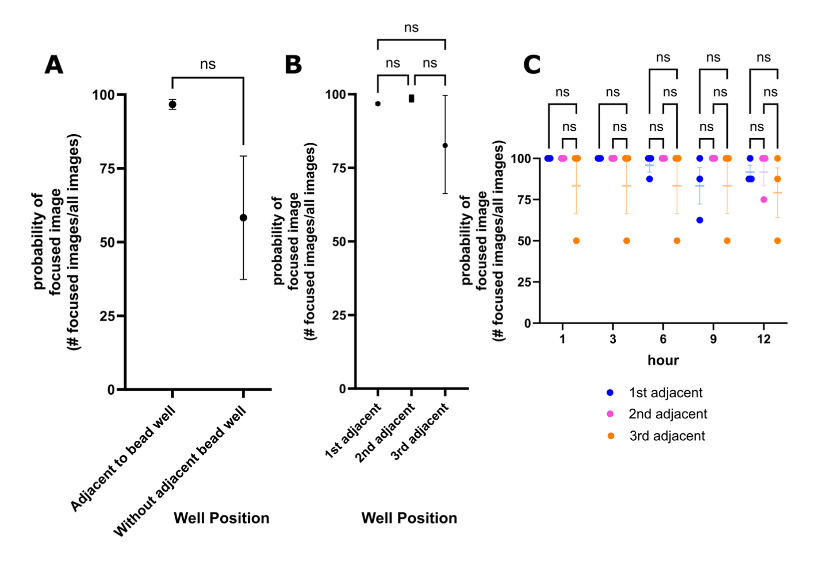
Figure 5. The presence of beads improves the reliability of obtaining a focused image with autofocus. The focus of images acquired in Experiment 2 was predicted using the image classifier in KNIME. For a detailed overview of the experimental setup, see Figure 2. Each point represents the probability of obtaining a focused image. The likelihood of obtaining a focused image was calculated from the number of focused images acquired and the total number of images acquired and was applied to all graphs. (A) The probability of a focused image when beads are scanned before adjacent wells (1st adjacent, 2nd adjacent, 3rd adjacent wells) and when images are acquired without a bead well (n = 1). Wells without beads were acquired before wells with beads in Experiment 2. Twenty images were analyzed from each repeat, generating a single data point each. The presence of a bead in a well improves the probability of obtaining a focused image at the first passage of the plate. (B) The position of the well with respect to a bead well and the probability of obtaining a focused image. Images from the complete 14-h scan were compiled to calculate the probability (n = 1). 4440, 4824, and 3216 images are the combined total images acquired across repeats. Image predictions were separated by well position and used to generate a single data point from each repeat. Regardless of the position of the well, obtaining a focused image is highly probable. (C) Hourly assessment of the probability of obtaining a focused image in all adjacent wells (n = 1). Images analyzed in panel B were separated by the time point. 48 images were analyzed for each category (i.e., 1st adjacent, 2nd adjacent, 3rd adjacent), representing 8 images analyzed at each timepoint. The presence of beads improves the consistency of acquiring a focused image in a long-term scan. Mann-Whitney was performed for panel A, Kruskal-Wallis was performed in panel B, and a two-way ANOVA was performed in panel C using GraphPad Prism (10.2.3). SEM bars are shown ns, P > 0.05; n = 3.
3. Efficacy of using distinct types of microbeads as a focus fiduciary
To determine if other beads could be used as a focus aid, fluorescent, non-fluorescent, and glass (silicon dioxide) microbeads were tested (Experiment 1, Figure 2A). All channels were used for autofocusing. The non-fluorescent beads appeared more prominently than the cells and exhibited strong autofluorescence (Figure 6). The non-fluorescent beads are larger than both the glass and fluorescent beads, and thus sit further above the plane of the cells than the smaller beads. The objective of adding the beads is to retain focus in long-term scans by preventing focal drift. We hypothesize that if the beads are much larger than the cells, this effect is lost as the autofocus is selecting a plane that is not the optimal focus position. Further, downstream segmentation of these images could be difficult, and the beads may be incorrectly identified as cell objects. The use of silicon dioxide beads produced hazy and low-contrast images compared to the other beads tested. In addition, a caveat of glass beads is that they can focus light by acting as ball lenses. Beads were used at three different dilutions (Figure 6). The effect of the beads in addressing prolonged well exposure and focal drift and preventing autofocus failures was evaluated at the highest dilution. In preliminary experiments, we found that this allowed for sufficient beads in each field to obtain the intended effect without compromising image appearance. It may be necessary to optimize bead dilution depending on cell dilution and objective magnification. Evaluation of the effects of the beads on cellular health was limited in the validation of this protocol. We did not observe, however, any evidence of interaction between the beads and cells (i.e., phagocytosis) or evident signs of detriment to cellular health.
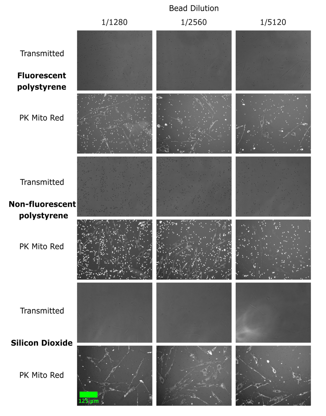
Figure 6. Example images of three distinct types of microbeads. Images have been acquired in Experiment 1. Fluorescent (Texas Red) polystyrene (PS) 2 μm, non-fluorescent polystyrene (PS) 3 μm, and non-fluorescent silica dioxide 2 μm microbeads were diluted to 1/1280, 1/2560, and 1/5120 (as listed on the top) into wells of a 384-well plate containing fibroblasts stained with PK Mito far red and media. The plate was centrifuged at 1,000× g for 5 min before imaging. Images were acquired using a 20× Plan fluorite objective on an EVOS M7000 microscope in brightfield and fluorescent mode. Autofocus was used in each channel. Scale bar, 125 μm.
General notes and troubleshooting
General notes
1. This protocol has been optimized for use with adherent cells.
2. In each experiment, the beads were diluted fresh. We found that diluting the beads and storing them in PBS resulted in aggregation (see Figure 7).
3. The exact procedure described above was used with the other beads evaluated in Experiment 1. Beads were further diluted for Experiment 1 than described in the procedure.
4. In all experiments, a well with beads was imaged before wells without beads (Figure 2). If the design of Experiment 2 is not followed, it is good practice to decide beforehand where the wells with beads will go, to ensure this can be done based on scanning options available on the microscope.
5. Autofocus was implemented by the EVOS software, which is used to control the microscope. The autofocus protocol described in the data acquisition section of the protocol was created using the Automate feature available on the EVOS software. The autofocus algorithm selected for all acquisitions is called fluorescence optimized. The algorithm is described in the EVOS manual as follows: “The focal plane is derived from the highest ratio between detailed, high-contrast objects against the background.”
6. This method has been evaluated solely on the EVOS imaging system.
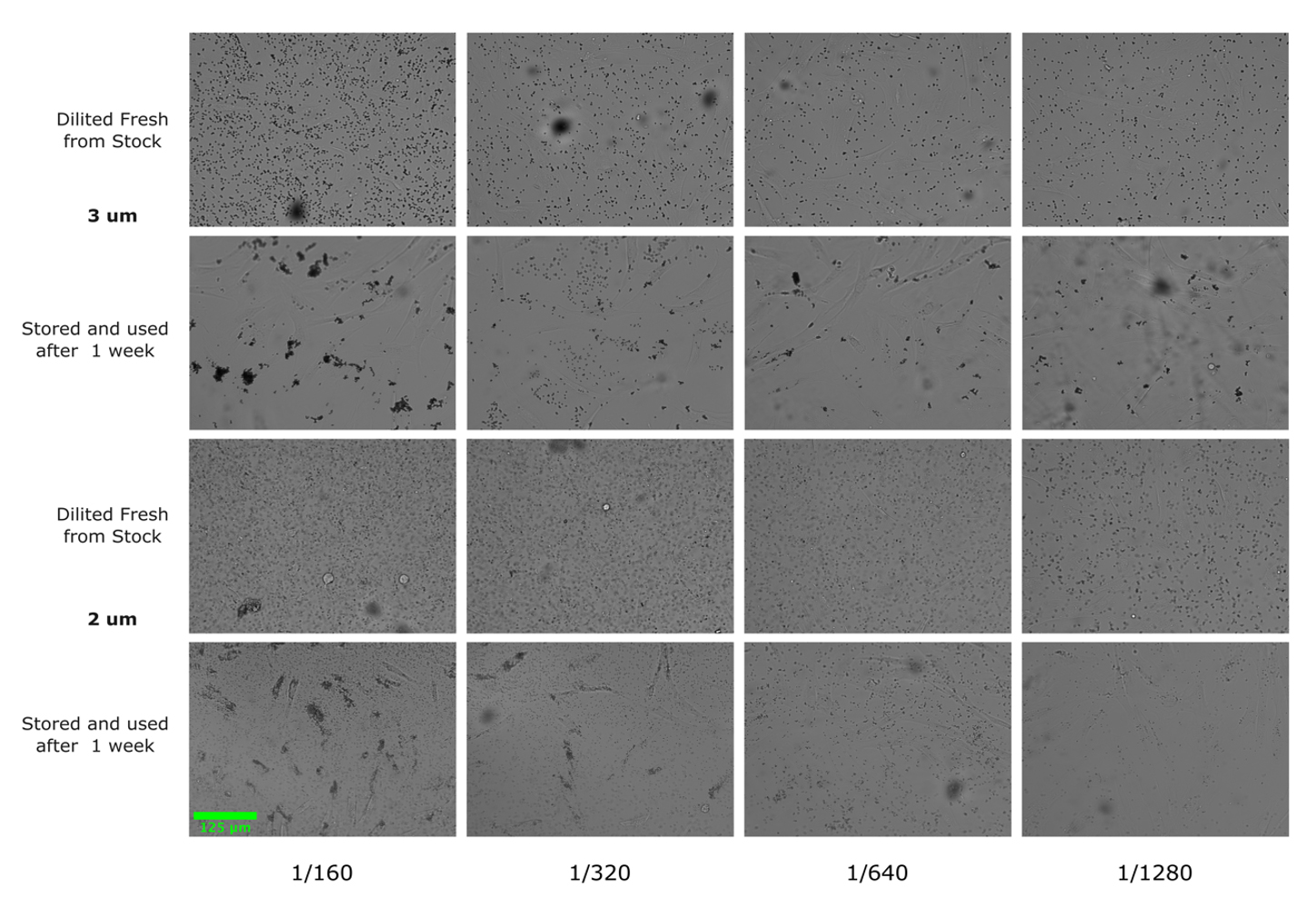
Figure 7. Beads diluted and stored in PBS aggregate over time. Images acquired on EVOS M7000 microscope using 20× Plan fluorite objective. Fluorescent (2 μm) and non-fluorescent (3 μm) beads were stored in 1.5 mL microcentrifuge tubes covered with foil at room temperature following dilution and are shown one week after storage. Results indicate beads should be diluted fresh with each experiment. Scale bar, 125 μm.
Acknowledgments
Conceptualization, R.T., E.J.O., and I.G.; Investigation, I.G. and E.J.O. Writing—Original Draft, I.G.; Writing—Review & Editing, I.G., E.J.O., and R.T.; Funding acquisition, R.T.; Supervision, R.T. Funding sources: Canadian National Science and Engineering Council.
Competing interests
The authors declare no conflicts of interest.
References
- Song, L., Hennink, E., Young, I. and Tanke, H. (1995). Photobleaching kinetics of fluorescein in quantitative fluorescence microscopy. Biophys J. 68(6): 2588–2600. https://doi.org/10.1016/s0006-3495(95)80442-x
- Ge, J., Wood, D. K., Weingeist, D. M., Prasongtanakij, S., Navasumrit, P., Ruchirawat, M. and Engelward, B. P. (2013). Standard fluorescent imaging of live cells is highly genotoxic. Cytometry Part A. 552–560. https://doi.org/10.1002/cyto.a.22291
- Milkovic, L., Cipak Gasparovic, A., Cindric, M., Mouthuy, P. A. and Zarkovic, N. (2019). Short Overview of ROS as Cell Function Regulators and Their Implications in Therapy Concepts. Cells. 8(8): 793. https://doi.org/10.3390/cells8080793
- Dixit, R. and Cyr, R. (2003) Cell damage and reactive oxygen species production induced by fluorescence microscopy: effect on mitosis and guidelines for non-invasive fluorescence microscopy. Plant J. 36(2):280–90. https://doi.org/10.1046/j.1365-313x.2003.01868.x
- Zheng, Q., Jockusch, S., Zhou, Z. and Blanchard, S. C. (2013). The Contribution of Reactive Oxygen Species to the Photobleaching of Organic Fluorophores. Photochem Photobiol. 90(2): 448–454. https://doi.org/10.1111/php.12204
- Sen, O., Saurin, A. T. and Higgins, J. M. G. (2018). The live cell DNA stain SiR-Hoechst induces DNA damage responses and impairs cell cycle progression. Sci Rep. 8(1): 7898. https://doi.org/10.1038/s41598-018-26307-6
- Mari, P. O., Verbiest, V., Sabbioneda, S., Gourdin, A. M., Wijgers, N., Dinant, C., Lehmann, A. R., Vermeulen, W. and Giglia-Mari, G. (2010). Influence of the live cell DNA marker DRAQ5 on chromatin-associated processes. DNA Repair. 9(7): 848–855. https://doi.org/10.1016/j.dnarep.2010.04.001
- Mubaid, F. and Brown, C. M. (2017). Less is More: Longer Exposure Times with Low Light Intensity is Less Photo-Toxic. Microsc Today. 25(6): 26–35. https://doi.org/10.1017/s1551929517000980
- Purschke, M., Rubio, N., Held, K. D. and Redmond, R. W. (2010). Phototoxicity of Hoechst 33342 in time-lapse fluorescence microscopy. Photochem Photobiol Sci. 9(12): 1634–1639. https://doi.org/10.1039/c0pp00234h
- Harada, T., Hata, S., Fukuyama, M., Chinen, T. and Kitagawa, D. (2022). An antioxidant screen identifies ascorbic acid for prevention of light-induced mitotic prolongation in live cell imaging. Commun Biol. 6(1):1107. https://doi.org/10.1101/2022.06.20.496814
- Harrison, P. J., Gupta, A., Rietdijk, J., Wieslander, H., Carreras-Puigvert, J., Georgiev, P., Wählby, C., Spjuth, O. and Sintorn, I. M. (2023). Evaluating the utility of brightfield image data for mechanism of action prediction. PLoS Comput Biol. 19(7): e1011323. https://doi.org/10.1371/journal.pcbi.1011323
- Bonet Sanz, M., Machado Sánchez, F. and Borromeo, S. (2021). An algorithm selection methodology for automated focusing in optical microscopy. Microsc Res Tech. 85(5): 1742–1756. https://doi.org/10.1002/jemt.24035
- Jia, D., Zhang, C., Wu, N., Zhou, J. and Guo, Z. (2022). Autofocus algorithm using optimized Laplace evaluation function and enhanced mountain climbing search algorithm. Multimedia Tools Appl. 81(7): 10299–10311. https://doi.org/10.1007/s11042-022-12191-w
- Redondo, R., Bueno, G., Valdiviezo, J. C., Nava, R., Cristóbal, G., Déniz, O., García-Rojo, M., Salido, J., Fernández, M. d. M., Vidal, J., et al. (2012). Autofocus evaluation for brightfield microscopy pathology. J Biomed Opt. 17(3): 036008. https://doi.org/10.1117/1.jbo.17.3.036008
- Geusebroek, J. M., Cornelissen, F., Smeulders, A. W. and Geerts, H. (2000). Robust autofocusing in microscopy. Cytometry. 39(1): 1–9. https://doi.org/10.1002/(sici)1097-0320(20000101)39:1<1::aid-cyto2>3.0.co;2-j
- Liu, S., Liu, M. and Yang, Z. (2016). An image auto-focusing algorithm for industrial image measurement. EURASIP J Adv Signal Process. 2016(1): 1–16. https://doi.org/10.1186/s13634-016-0368-5
- Mateos‐Pérez, J. M., Redondo, R., Nava, R., Valdiviezo, J. C., Cristóbal, G., Escalante‐Ramírez, B., Ruiz‐Serrano, M. J., Pascau, J. and Desco, M. (2012). Comparative evaluation of autofocus algorithms for a real‐time system for automatic detection of Mycobacterium tuberculosis. Cytometry Part A. 81(3): 213–221. https://doi.org/10.1002/cyto.a.22020
- Hung, C. K., Maiuri, T., Bowie, L. E., Gotesman, R., Son, S., Falcone, M., Giordano, J. V., Gillis, T., Mattis, V., Lau, T., et al. (2018). A patient-derived cellular model for Huntington’s disease reveals phenotypes at clinically relevant CAG lengths. Mol Biol Cell. 29(23): 2809–2820. https://doi.org/10.1091/mbc.e18-09-0590
- Barba Bazan, C., Goss, S., Peng, C., Begeja, N., Suart, C., Neuman, K. and Truant, R. (2021). Mod3D: A Low-Cost, Flexible Modular System of Live-Cell Microscopy Chambers and Holders. bioRxiv: e462400. https://doi.org/10.1101/2021.10.18.462400
Article Information
Publication history
Received: Nov 21, 2024
Accepted: May 26, 2025
Available online: Jul 11, 2025
Published: Jul 20, 2025
Copyright
© 2025 The Author(s); This is an open access article under the CC BY-NC license (https://creativecommons.org/licenses/by-nc/4.0/).
How to cite
Gibson, I., Osterlund, E. J. and Truant, R. (2025). Using Beads as a Focus Fiduciary to Aid Software-Based Autofocus Accuracy in Microscopy. Bio-protocol 15(14): e5388. DOI: 10.21769/BioProtoc.5388.
Category
Cell Biology > Cell imaging > Live-cell imaging
Do you have any questions about this protocol?
Post your question to gather feedback from the community. We will also invite the authors of this article to respond.