Two-photon (2P) Microscopy to Study Ca²⁺ Signaling in Astrocytes From Acute Brain Slices

Materials and reagents

Biological materials

1. Adeno-associated viral (AAC) vectors:

a. AAV5.GfaABC1D.tdTomato.SV40 (Penn Vector Core, Addgene 44332; MTA required by Addgene)

b. AAV5.GfaABC1D.cyto-GCaMP6f.SV40 (Penn Vector Core, Addgene 52925; MTA required by Addgene)

b. AAV5.GfaABC1D.G-CEPIA1er.SV40 [this plasmid is not commercially available; it was kindly donated by Dr. Y. Okubo (Department of Pharmacology, Graduate School of Medicine, University of Tokyo). Note that a virus packaging service is needed to insert the plasmid into the AAV5 vector].

Note: Store AAVs at -80 °C upon arrival. Prepare aliquots of appropriate volume (e.g., 3–5 μL) from the delivered batch to avoid freezing/thawing cycles.

Critical: Use a minimum titer of 1–2 × 10¹³ vg/mL.

Reagents

1. Phosphate buffer saline (PBS), sterile-filtered, pH 7.4 (Merck, catalog number: P4474)

2. Carprofen (Rimadyl, Pfizer, USA)

3. Eye ointment (Paralube ophthalmic ointment or similar, e.g., Lubrithal)

3. Povi-iodine 100 (Farmec srl) or similar (e.g., Betadine)

4. Isoflurane (Iso-Vet, Boehringer Ingelheim Animal Health Italia S.p.A)

5. Glucose (Merck, catalog number: G7528)

6. NaCl (Merck, catalog number: S7653)

7. KCl (Merck, catalog number: P9333)

8. NaHCO₃ (Merck, catalog number: S5761)

9. NaH₂PO₄ (Merck, catalog number: S3139)

10. MgCl₂ (Merck, catalog number: M2670)

11. CaCl₂ (Merck, catalog number: 21115)

12. K-Gluconate (Merck, catalog number: P1847)

13. EGTA (Merck, catalog number: E4378)

14. HEPES (Merck, catalog number: H3375)

15. D-Mannitol (Merck, catalog number: M4125)

Note: Chemicals and salts may also be purchased from other companies.

Solutions

1. Standard solution (see Recipes)

2. Gluconate solution (see Recipes)

3. Mannitol solution (see Recipes)

4. Recording solution (see Recipes)

Recipes

1. Standard solution (final volume of 500 mL)

Reagent	Final concentration	Quantity or volume
Glucose	25 mM	2.253 g
NaCl 2 M	125 mM	31.25 mL
KCl 2 M	2.5 mM	0.625 mL
NaHCO3 0.5 M	25 mM	25 mL
NaH2PO4 1 M	1.25 mM	0.625 mL
MgCl2 1 M	1 mM	0.5 mL
CaCl2 1 M	2 mM	1 mL

Note: Bring to a final volume of 500 mL with MilliQ water and keep the solution on ice. Before adding CaCl₂, bubble the solution for at least 20 min with 95% O₂ and 5% CO₂ to reach pH 7.4 and prevent CaCl₂ precipitation. Keep constantly bubbled throughout the preparation. Prepare fresh before use. A 10× stock solution (500 mL) can be prepared without glucose, MgCl₂, and CaCl₂. Store the 10× solution at 4 °C and use it within 1 month.

2. Gluconate solution (2 L stock)

Reagent	Final concentration	Quantity or volume
Glucose	25 mM	9.01 g
K-Gluconate	130 mM	60.9 g
KCl	15 mM	2.24 g
EGTA	0.2 mM	0.152 g
HEPES	20 mM	9.53 g

Note: Adjust the pH to 7.4 with NaOH and bring to a final volume of 2 L. This solution can be prepared in advance as 1× stock and frozen at -20 °C in 50 mL tubes for up to 6 months. On the day of the experiment, you will need 100 mL of solution; thus, thaw two aliquots and keep the solution on ice under 99.95% O₂ bubbling for at least 45 min before use. Keep the solution bubbled with 99.95% O₂ throughout the procedure to ensure proper oxygenation of the tissue. Since this solution is buffered with HEPES and not with NaHCO₃, it does not require CO₂ bubbling.

3. Mannitol solution (final volume of 100 mL)

Reagent	Final concentration	Quantity or volume
Glucose	25 mM	0.45 g
D-Mannitol	225 mM	4.1 g
KCl 2 M	2.5 mM	0.125 mL
NaHCO3 0.5 M	26 mM	5.2 mL
NaH2PO4 1 M	1.25 mM	0.125 mL
MgCl2 1 M	8 mM	0.8 mL
CaCl2 1 M	0.8 mM	0.08 mL

Note: Bring to a final volume of 100 mL with MilliQ water. Before adding CaCl₂, bubble the solution for at least 20 min with 95% O₂ (ensure proper oxygenation of the tissue) and 5% CO₂ to reach pH 7.4, thus preventing CaCl₂ precipitation. Keep constantly bubbled at room temperature throughout the preparation. Prepare fresh before use. A 10× stock solution (500 mL) can be prepared without glucose, mannitol, MgCl₂, and CaCl₂. Store the 10× solution at 4 °C and use it within 1 month.

4. Recording solution (500 mL)

Reagent	Final concentration	Quantity or volume
Glucose	10 mM	0.9 g
NaCl 2 M	120 mM	30 mL
KCl 2 M	2.5 mM	0.625 mL
NaHCO3 0.5 M	26 mM	26 mL
NaH2PO4 1 M	1.25 mM	0.625 mL
MgCl2 1 M	1 mM	0.5 mL
CaCl2 1 M	1 mM	0.5 mL

Note: Bring to a final volume of 500 mL with MilliQ water. Before adding CaCl₂, bubble the solution for at least 20 min with 95% O₂ and 5% CO₂ to reach pH 7.4 and prevent CaCl₂ precipitation. Keep constantly bubbled throughout the preparation. Prepare fresh before use. Keep the solution at room temperature.

Laboratory supplies

1. Surgery tools: scissors, forceps, tweezers, suture thread [Fine Science Tools: catalog number: 14060-09 (fine scissors, sharp), 11210-10 (Dumont AA, epoxy-coated forceps), 15018-10 (Vannas spring scissors, Ethicon), 8697 6-0 (Prolene suture thread)]

2. Glass capillaries (pipettes) (Narishige, catalog number: GD-1)

3. Drill burs (Meisinger, catalog number: 1RF-007; Fine Science Tools, catalog number: 19008-07 SS 0.7 mm, round HP Burs)

4. Cotton swabs

5. Beakers (50 mL and 100 mL)

6. Bottles (100 mL and 500 mL) for saline solutions

Equipment

1. Freezer -80 °C (Thermo Scientific, model: Revco ExF)

2. Freezer -20 °C (Liebherr, model: SFFvh 4001 Perfection)

3. Refrigerator 4 °C (Liebher, model: SRFfg 3501 Performance)

4. Thermostatic bath (ISCO, model: GTR-90)

5. Pure O₂ tank (AirLiquide, Oxygen purity ≥ 99,995%)

6. 5% CO₂/95% O₂ tank (AirLiquide)

7. Pipette puller (Narishige, Japan, model: PC-10)

8. Anesthesia unit for isoflurane (anesthesia system, lab animal, complete, V-1 tabletop with active scavenging) (KF Technology, model: 901820)

9. Heating pad with controller (Stoelting, model: 53800M)

10. Digital stereotaxic apparatus (digital just for mouse stereotaxic instrument) (Stoelting, model: 51730D)

11. Stereomicroscope (Leica, model: CLS150MR)

12. Dental drill (Sifradent, model: MM 330VPR)

13. Heat lamp (Braintree Scientific Inc., model: MM 330VPR); as a general recommendation, use an infrared heat lamp with a 150–250 W bulb and an adjustable swing arm for easy adjustment of the distance to the animal. The animal should have the possibility to move away to a non-heated part of the cage

14. Vibratome (Leica BioSystems, model: VT1200)

15. Dual Fluorescent Protein Flashlight kit, including barrier filter glasses (NightSea, now replaced by Xite Flashlight System)

16. 2-photon laser scanning microscope (Multiphoton Imaging System, Scientifica Ltd., UK) equipped with a water-immersion objective (LUMPlan FI/IR 20×, 1.05 NA, Olympus), a pulsed mode locked Ti:Sapphire laser (Chameleon Ultra 2, Coherent, USA) and a Pockels cell for laser power modulation (ConOptics, USA, model: 302RM)

17. Peristaltic pump (Ismatec ISM831C Reglo Digital Variable-Speed Peristaltic Pump 2 Channel)

Software and datasets

1. SciScan (Scientifica UK, version 1.2, included with Scientifica 2-photon system) for image acquisition

2. ImageJ (publicly available at https://github.com/imagej/ImageJ, we used version 1.51n) for image analysis

3. GECI Quant script (see https://baljitkhakhlab.healthsciences.ucla.edu/tools) for ROI detection in ImageJ

4. AstroResp Code (publicly available at https://github.com/ladymariot/AstroResp) for peak detection, extraction of fluorescent traces, and peak parameters

5. MATLAB 7.6.0 R2008 A (Mathworks, Natick, MA, USA) for running AstroResp Code

6. Excel (Microsoft Office Professional 2016, OpenOffice Calc as a free alternative) for data handling

7. OriginPro (OriginLab, version 2018, QtiPlot as a free alternative) for trace analysis and graph production

Procedure

A. Intracortical AAV injection in the mouse somatosensory cortex

Notes:

1. After practical training, the whole procedure takes approximately 40 min per mouse.

2. To obtain significant data, around 6 mice per experimental condition are generally needed.

Caution: Carefully follow all directives for procedures involving viral vector handling in your facility.

1. Prepare a glass pipette by using the pipette puller. Set the puller temperature for a tip diameter of 35–45 μm.

2. By using graph paper as a guide, with a fine marker, draw notches spaced 2 mm on the glass capillary; each notch will correspond to 0.5 μL.

3. Prepare the mix of AAVs by using 60% of GCaMP6f (or G-CEPIA1er) and 40% of tdTomato. Use AAVs with a titer in the order of 1–2 × 10¹³. Keep the mix on ice. For each mouse, you will need 1.5 μL of mix. Adjust the mix volume depending on the number of mice to be injected in the session.

Note: The amount of mix is irrespective of the age and weight of the mouse. This procedure has been validated in mice from 1 to 12 months of age.

4. Prepare your workspace for surgery and sterilize surgery equipment (Figure 1A–B).

5. Connect the glass pipette to the stereotaxic arm of the apparatus (Figure 1C).

6. Check the mouse body weight; it should be above 15 g.

7. Anesthetize the mouse with 4% isoflurane/1.5% oxygen flow in the induction chamber (Figure 1D–E).

8. Once the mouse is deeply anesthetized, gently move it to the stereotaxic apparatus and maintain anesthesia with the dedicated mask (Figure 1F) but lower isoflurane to 1.5% while keeping the 1.5% oxygen flow constant. Assure anesthesia depth by monitoring respiration rate, eyelid reflex, vibrissae movements, and reactions to tail and toe pinching. Keep the animal warm on a controlled heating pad set at 37 °C for the entire procedure.

9. Subcutaneously inject Carprofen (5 mg/kg) to reduce pain.

10. Ensure that the head of the mouse is well fixed to the stereotaxic apparatus (Figure 1F).

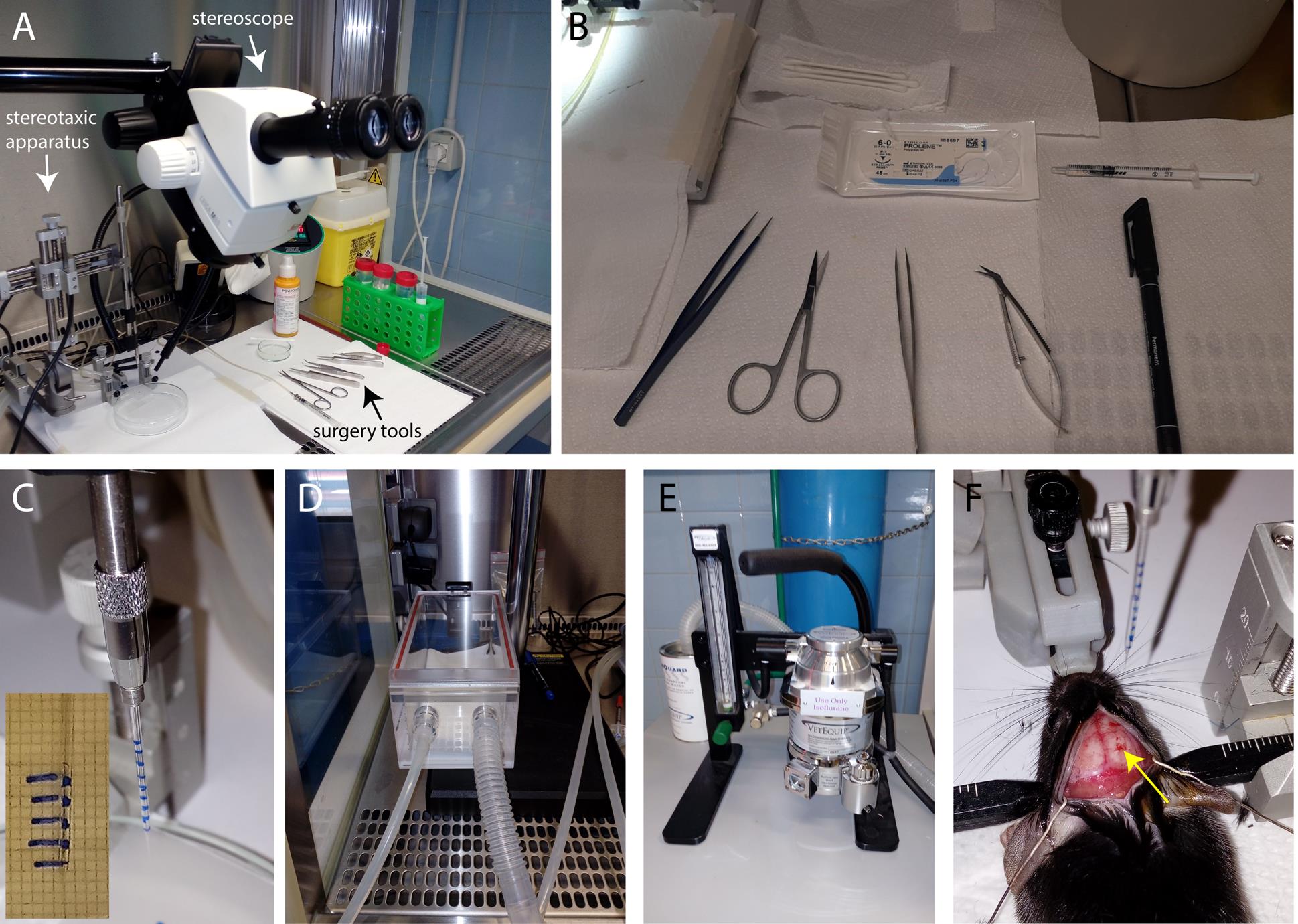
Figure 1. Preparation for stereotaxic intracortical injections. (A) Stereotaxic apparatus, stereoscope, and surgical tools (arrows) are prepared under the BL2 hood. (B) Surgical tools, marker, suture thread, and 1 mL syringe with PBS. (C) Glass capillary with marked notches is positioned on the stereotaxic holder. The inset shows the graph paper used for capillary labeling. (D) Anesthesia induction chamber. (E) Anesthesia vaporizer. (E) The mouse head is fixed in the stereotaxic apparatus, the brain is exposed, and the viral mix-loaded capillary is ready to be lowered for injection (yellow arrow points to the drilled site).

11. Apply eye ointment to prevent eye drying.

12. Remove hair from the head using scissors. You can also use a rodent trimmer.

13. Clean the skin with Povi-iodine 100.

14. Cut the scalp using sharp, straight scissors with a cutting edge of 22 mm, starting from above the cerebellum and finishing in between the eyes.

15. Open the scalp to expose the skull.

16. Clean the skull by using a cotton swab and forceps. Remove all the periosteum membranes.

17. Level the skull along the anterior-posterior axis by using the bregma and lambda as reference points. The delta between them should be less than 0.3 mm in the dorso-ventral direction.

18. Level the skull along the medio-lateral axis: +/-2 mm relative to bregma. Also, in this case, the delta between +2 from the bregma and -2 from the bregma should be less than 0.3 mm.

19. With a marker, sign the two injection sites in the somatosensory cortex using the stereotaxic coordinates. Move the tip of the capillary on the bregma and set all coordinates to zero in the digital coordinate apparatus. For the first hole, consider: 0.5 mm posterior to the bregma and 1.5 mm lateral to the bregma. For the second hole, consider: 1.5 mm posterior to the bregma and 1 mm lateral to the bregma.

20. Using the dental drill, drill small holes at both injection sites (approximately 0.2 mm diameter).

Critical: Try to avoid bleeding from the brain during drilling by keeping the dura mater intact.

21. During drilling, pause frequently to wash the skull with one drop of sterile-filtered PBS to reduce overheating, then dry it with a cotton swab before restarting drilling.

22. Make sure to blow away any debris or bone pieces above the injection site after drilling.

23. After drilling both holes, load the glass capillary. Prepare a piece of parafilm on a Petri dish and put 1.5 μL of AAV mix on it. Ensure that the capillary tip is touching the liquid, then pull the viral mix by exerting low pressure on the syringe. Once the mix starts to move up, do not increase the pressure. To stop the suction, remove the syringe from the tube.

24. Position the virus-loaded glass capillary above the first injection hole, touch the brain surface with the capillary tip, and set the zero position on the Z-axis.

25. Lower the capillary tip to -0.6 μm depth and inject 0.25 μL of virus. Be sure to use as low pressure as possible (0.25 μL should be injected in 30 s) to avoid the virus spilling over the tissue. Wait by leaving the tip in the same position for 3 min, to let the virus diffuse.

26. Raise the tip to -0.4 μm and inject 0.25 μL of virus. Again, be sure to use as low pressure as possible and leave the tip in the same position for 3 min.

27. Raise the tip to -0.3 μm and inject 0.25 μL of virus with low pressure. Leave the tip in the same position for 5 min to let the virus diffuse, then remove the tip from the hole.

28. Repeat steps A25–27 for the second hole. Remove the tip from the hole.

29. Humidify the skin with sterile-filtered PBS.

30. Suture the skin by using forceps and suture thread and adding a minimum of two suture points. If necessary, add other suture points. Clean the wound with 200 µL of Povi-iodine 100.

31. Return the mouse to the home cage under the heat lamp and let it wake up.

32. Wait between 2 and 3 weeks after injection before proceeding with brain slice preparation.

B. Cortical brain slice preparation

Note: After practical training, the whole procedure of cortical brain slice preparation from step B6 to B18 takes approximately 40 min + recovery time.

1. Put the slicer chamber, a glass Petri dish, an 80 mL beaker (beaker 1), and a 50 mL beaker (beaker 2) at -20 °C, all covered with parafilm, for 30 min before starting the procedure.

2. Keep the gluconate solution (under 99.5% O₂ bubbling) and the standard solution (under 95% CO₂ and 5% O₂ bubbling) on ice. Gluconate solution is essentially devoid of Ca²⁺ and Na⁺ ions, mimicking the intracellular medium. The aim is to limit the entry of extracellular ions into cells whose processes are cut during slicing, thus avoiding excitotoxicity.

3. Prepare two 100 mL beakers with a net to hold the slices (built with a 50 mL tube cap and fiberglass net; see Figure 2A–B). Keep one at room temperature with Mannitol solution and the other in the thermostatic bath at 32 °C with standard solution, both under 95% CO₂ and 5% O₂ bubbling. Mannitol solution is an intermediate solution in which Na⁺ and Ca²⁺ concentrations are partially increased. The rationale is that slices undergo gradual adjustments of extracellular ionic composition from gluconate to standard solution.

4. Put the cold slicer chamber in the slicer, filling it with ice.

5. Fill the glass Petri dish, beaker 1, and beaker 2 with cold standard solution. Put beaker 2 on ice and keep the solutions continuously bubbled with 95% CO₂ and 5% O₂.

6. Anesthetize the mouse with 4% isoflurane or by putting one drop of isoflurane on a piece of paper inside the cage.

7. Once the mouse is deeply anesthetized (1–2 min), cut the head and place it in beaker 1 with ice-cold standard solution.

8. Using the tweezers, transfer the head from beaker 1 to the glass Petri dish.

9. Hold firmly the head by the nose using the tweezers, take the scissors, and remove the scalp.

10. Remove the brain. Be careful during extraction to avoid damaging it.

Critical: The extraction of the brain must be done carefully but as fast as possible, to minimize damage due to lack of oxygenation to the tissue.

11. Transfer the brain to beaker 2 and keep it bubbled with 95% CO₂ and 5% O₂.

12. Fill the slice chamber with gluconate solution and keep it bubbled with pure O₂.

13. Place the brain on a Petri dish and check tdTomato expression using the Dual Fluorescent Protein Flashlight (use green light and wear red glasses).

14. Cut the cerebellum with a blade.

15. Glue the brain, on the caudal site, to the vibratome metal plate.

16. Transfer the vibratome metal plate to the slice chamber and orient the brain with the cortex toward the blade.

17. Cut 350 μm slices within the somatosensory cortex area (check the probe expression on the slice with the Dual Fluorescent Protein Flashlight).

18. Transfer individual slices in the beaker with the net containing mannitol solution and keep the slices there for 1 min.

19. After 1 min, transfer slices to the other beaker with the net containing standard solution at 32 °C for 20 min.

20. Transfer the beaker with the slices to room temperature and let the slices recover for at least 1 h before starting experiments. This time helps brain slices to recover after the stress of the slicing procedure.

Note: These slices are vital for 4–5 h after recovery. Always check for cellular morphology with brightfield microscopy at the beginning of the experiment to recognize changes and signs of poor vitality (such as swollen neurons or evidence of round, expanded nuclei).

C. 2-photon laser scanning microscope imaging

Caution: Follow carefully all safety procedures related to Laser Class 4. Wear appropriate DPIs (e.g., protective goggles).

1. Turn on the laser at least 3 h before the experiment, in order to stabilize beam radiation. In case a Pockels cell is included in the path, open the laser shutter to allow warming up and stabilization of the internal components.

2. Prepare the perfusion system by pre-filling it with recirculating recording solution, and adjust the speed to 3 mL/min (Figure 2C). Always keep the solution source (typically, a 50 mL tube) under bubbling and avoid excessively long tubing to minimize oxygenation changes. Typically, the time taken for the solution to travel from the source to the chamber is between 30 and 60 s.

3. After the recovery time for brain slices, place one slice in the submerged perfusion chamber under the objective and gently put the platinum wire anchor with nylon strands over the slice to hold it still (Figure 2D).

4. Use widefield imaging under a green fluorescence source (LED or lamp) to focus and localize the site of tdTomato probe expression in the somatosensory cortex using the binoculars or with a connected camera. Start with a 4× objective, if possible, to have a wider view of the slice, then replace with a 20× objective.

Caution: During acquisition with 2PLSM, keep the room in complete darkness to protect photon detectors.

5. Set the laser wavelength to 920 nm to excite both GCaMP6f (or G-CEPIA1er) and tdTomato. Emission fluorescence can be collected in two different channels (Figure 2E–F). We use a filter cube with a 565 nm dichroic filter and two emission filters for green and red channels (525/50 and 620/60 nm, respectively).

6. We suggest using a zoom factor of 2.5× in order to acquire 1–3 astrocytes with a sufficient resolution in a field of view of 120 μm × 120 μm. Set the resolution to 512 × 512 pixels. Power at the sample should be kept at 10–15 mW, but always under 20 mW to avoid photo-stimulation.

7. Choose focal planes at 60–80 μm depth to avoid imaging possible unhealthy cells at superficial planes. Use tdTomato fluorescence to identify and focus AAV-infected astrocytes and choose astrocytes with a low GCaMP6f signal at rest. Acquire the signals for 1–2 min to check for astrocyte spontaneous activity and GCaMP6f expression.

8. For G-CEPIA1er-expressing astrocytes, the choice of field of view is easier because the fluorescence of this probe is high at resting Ca²⁺ concentrations in the endoplasmic reticulum.

9. Once the field of view is selected, perform recording sessions of 2 min with a 5 min interval between successive acquisitions to avoid photo-stimulation. Acquire at least two time series in basal (non-stimulated) conditions. Before each recording, check and correct the focus using tdTomato fluorescence as a reference.

10. To extract information on astrocyte activity that is independent of neuronal action potential firing, it is possible to block voltage-gated Na⁺ channels by perfusing the slices with tetrodotoxin (TTX). Perfuse with TTX 0.5 μM in recording solution for at least 10 min and repeat two acquisitions of basal signal, always in the presence of TTX.

11. To extract information on astrocyte signals upon metabotropic agonist stimulation, prepare 50 mL of recording solution with the appropriate agonist concentration (for example, 10 μM Noradrenaline), always in TTX 0.5 μM. Acquire a T-series of 3 min to allow capturing astrocyte response to metabotropic receptor activation. In case of necessity, acquire a second T-series to capture the end of the astrocyte response. Wash with 50 mL of recording solution before the next experiment.

Note: While 3 min is generally sufficient to record the dynamics of the cytosolic response, the ER signal has a much slower recovery, enabling the visualization of Ca²⁺ release from the ER but not its refilling.

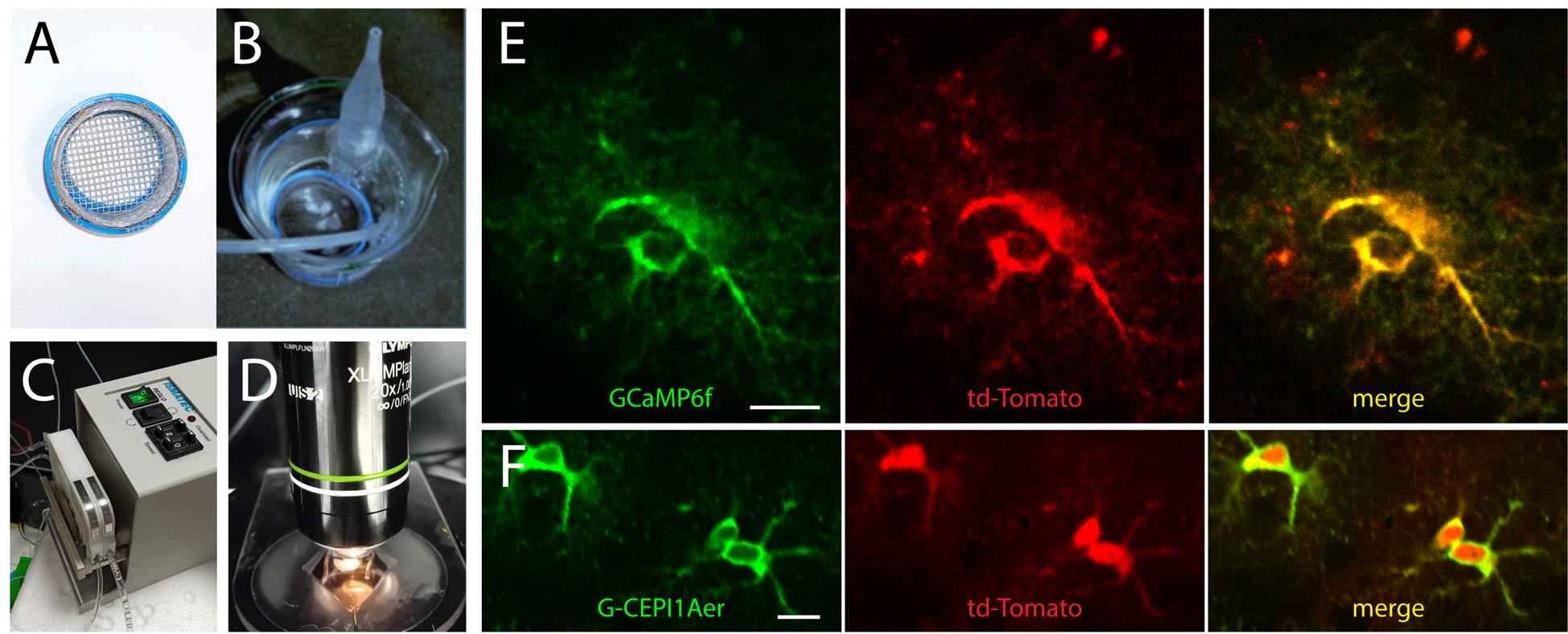
Figure 2. 2-photon imaging of intracellular Ca²⁺ signal in astrocytes. (A) Net for slices. (B) Brain slices in the beaker with the net, in standard solution under O₂/CO₂ bubbling. (C) Peristaltic pump for recording solution perfusion. (D) Perfusion chamber with a brain slice under the platinum grid in the 2P microscope setup, under a 20× objective. (E) Representative 2P images (average projection of 180 frames) of two SSCx astrocytes expressing GCamp6f and tdTomato. (F) Representative 2P images (average projection of 180 frames) of three SSCx astrocytes expressing CEPIA1er and tdTomato. Scale bar, 10 μm.

Data analysis

Analysis of fluorescence data from GCaMP6f and CEPIA1er-expressing astrocytes in basal conditions and upon receptor stimulation are detailed in the Methods section of our original research paper (Lia et al. 2023 [14]) and in the README file included in the public folder of AstroResp Code (https://github.com/ladymariot/AstroResp), where sample images are also provided to allow testing the code.

Briefly, GCaMP6f astrocyte fluorescence is analyzed and separately extracted for somata, principal processes, and microdomains. The use of the semi-automatic GECI Quant script [15] allows the identification of the different regions of interest (ROIs) based on their dimension and fluorescence intensity, while ImageJ software extracts the time course of the mean fluorescence value of pixels composing individual ROIs. A custom MATLAB script (AstroResp, originally described in [16]) normalizes fluorescence dynamics by calculating ΔF/F₀, then it identifies potential peaks in ΔF/F₀ traces by combining different thresholds referred to as global and local signal baselines. A final step of visual inspection allows the operator to manually discard traces dominated by noise. The astrocyte responses can be compared between different experimental conditions in relation to different extracted parameters, such as the amplitude and the frequency of responses at different compartments, or the number of active microdomains per astrocyte.

G-CEPIA1er fluorescence is analyzed by manually drawing an ROI in the somatic compartment and extracting the time course of the signal with ImageJ software. It is possible to normalize the change in fluorescence signal upon metabotropic stimulation (which induces a signal drop due to Ca²⁺ release from the ER) to basal values. To obtain hints about a possible difference in resting ER Ca²⁺ levels, we suggest analyzing a high number of cells (in the order of hundreds) in at least three mice per group, and also measuring tdTomato fluorescence in the different groups to check for uniformity of infection level.

Regarding statistical analysis, we compare two sample data sets with a Student’s t-test on normally distributed data and a Mann–Whitney test on non-normally distributed data.

Validation of protocol

This protocol (or parts of it) has been used and validated in the following research articles:

1. Lia et al. [14]. Rescue of astrocyte activity by the calcium sensor STIM1 restores long-term synaptic plasticity in female mice modelling Alzheimer’s disease. Nat Commun.

2. Mariotti et al. [16]. Interneuron-specific signaling evokes distinctive somatostatin-mediated responses in adult cortical astrocytes. Nat Commun.

3. Speggiorin et al. [17]. Characterization of the astrocyte calcium response to norepinephrine in the ventral tegmental area. Cells.

4. Requie et al. [18]. Astrocytes mediate long-lasting synaptic regulation of ventral tegmental area dopamine neurons. Nature Neurosci.

General notes and troubleshooting

General notes

1. This protocol describes experimental procedures for the mouse somatosensory cortex but is also applicable to other brain regions with appropriate modifications (e.g., stereotaxic coordinates for AAV injection and sectioning plane at the vibratome). See, for example, [17] for 2P imaging of astrocytes in the ventral tegmental area.

2. We recommend confirming cell specificity and extent of AAV expression in your preparation by performing immuno-histochemical characterization of protein expression in the different brain cell types, as in [16].

Troubleshooting

1. During intracortical injection of the viral mix, it may happen that the capillary tip gets plugged and, consequently, the virus cannot be injected. In this case, extract the capillary from the tissue and break off the very tip using tweezers. If this is not sufficient, use a new glass capillary.

2. If Ca²⁺ traces are dominated by noise, try to increase the gain of 2-photon microscope photomultiplier tubes (PMTs). Do not exceed the value where noise starts increasing more than the signal. In general, gallium arsenide phosphide detectors (GaAsPs) provide a higher signal/noise ratio compared to multialkali PMTs.

Acknowledgments

Specific contributions of each author: Conceptualization, Writing-Original Draft and Review & Editing, M.Z. and A.L.; Supervision, M.Z.

Funding sources that supported the original work related to this protocol: PRIN-20175C22WM to C.F.; Fondazione Cassa di Risparmio di Padova e Rovigo (CARIPARO Foundation) Excellence project 2017 (2018/113) to T.P. and G.C.

The authors acknowledge Euro-BioImaging ERIC (https://ror.org/05d78xc36) for providing access to imaging technologies and services via the Advanced Light Microscopy Node in Padova, Italy (https://ror.org/00h3qhh74).

The original research paper in which the protocol was described and validated is [14].

We are grateful to Dr. Gabriele Losi for the images of mouse surgery and slice recovery beaker, and Dr. Marta Gómez-Gonzalo for the image of the slice perfusion chamber.

Part of the graphical overview was created with BioRender: Lia, A. (2025) https://BioRender.com/im1epib.

Competing interests

The authors declare no conflicts of interest.

Ethical considerations

All experimental procedures were performed according to the European Committee guidelines (decree 2010/63/CEE) and the Animal Welfare Act (7 USC 2131), in compliance with the ARRIVE guidelines, and were approved by the Animal Care Committee of the University of Padua and the Italian Ministry of Health (authorization decrees 461/2017-PR, 929/2016-PR and 789/2019-PR).

References

1. Oliveira, J. F. and Araque, A. (2022). Astrocyte regulation of neural circuit activity and network states. Glia. 70(8): 1455–1466. https://doi.org/10.1002/glia.24178
2. Lyon, K. A. and Allen, N. J. (2021). From synapses to circuits, astrocytes regulate behavior. Front Neural Circuits. 15: 786293. https://doi.org/10.3389/fncir.2021.786293
3. Barros, L. F., Schirmeier, S., Weber, B. (2024). The astrocyte: Metabolic hub of the brain. Cold Spring Harb Perspect Biol. 16: a041355. https://doi.org/10.1101/cshperspect.a041355
4. Lee, H-G., Wheeler, M. A., Quintana, F. J. (2022). Function and therapeutic value of astrocytes in neurological diseases. Nat Rev Drug Discov. 21: 339–358. https://doi.org/10.1038/s41573-022-00390-x
5. Lia, A., Henriques, V. J., Zonta, M., Chiavegato, A., Carmignoto, G., Gómez-Gonzalo, M. and Losi, G. (2021). Calcium signals in astrocyte microdomains, a decade of great advances. Front Cell Neurosci. 15: 673433. https://doi.org/10.3389/fncel.2021.673433
6. Araque, A., Carmignoto, G., Haydon, P. G., Oliet, S. H. R., Robitaille, R. and Volterra, A. (2014). Gliotransmitters travel in time and space. Neuron. 81(4): 728–739. https://doi.org/10.1016/j.neuron.2014.02.007
7. Reeves, A. M. B., Shigetomi, E. and Khakh, B. S. (2011). Bulk loading of calcium indicator dyes to study astrocyte physiology: key limitations and improvements using morphological maps. J Neurosci. 31(25): 9353–9358. https://doi.org/10.1523/JNEUROSCI.0127-11.2011
8. Wahis, J., Baudon, A., Althammer, F., Kerspern, D., Goyon, S., Hagiwara, D., Lefevre, A., Barteczko, L., Boury-Jamot, B., Bellanger, B., et al. (2021). Astrocytes mediate the effect of oxytocin in the central amygdala on neuronal activity and affective states in rodents. Nat Neurosci. 24(4): 529–541. https://doi.org/10.1038/s41593-021-00800-0
9. Nanclares, C., Poynter, J., Martell-Martinez, H. A., Vermilyea, S., Araque, A., Kofuji, P., Lee, M. K. and Covelo, A. (2023). Dysregulation of astrocytic Ca²⁺ signaling and gliotransmitter release in mouse models of α-synucleinopathies. Acta Neuropathol. 145(5): 597–610. https://doi.org/10.1007/s00401-023-02547-3
10. Shigetomi, E., Bushong, E. A., Haustein, M. D., Tong, X., Jackson-Weaver, O., Kracun, S., Xu, J., Sofroniew, M. V., Ellisman, M. H. and Khakh, B. S. (2013). Imaging calcium microdomains within entire astrocyte territories and endfeet with GCaMPs expressed using adeno-associated viruses. J Gen Physiol. 141(5): 633–647. https://doi.org/10.1085/jgp.201210949
11. Stobart, J. L., Ferrari, K. D., Barrett, M. J. P., Glück, C., Stobart, M. J., Zuend, M. and Weber, B. (2018). Cortical circuit activity evokes rapid astrocyte calcium signals on a similar timescale to neurons. Neuron. 98(4): 726–735.e4. https://doi.org/10.1016/j.neuron.2018.03.050
12. Kuchibhotla, K. V., Lattarulo C. R., Hyman B. T. and Backsai B. J. (2009). Synchronous hyperactivity and intercellular calcium waves in astrocytes in Alzheimer mice. Science. 323(5918):1211–5. https://doi.org/10.1126/science.1169096.
13. Asrican, B., Wooten, J., Li, Y.-D., Quintanilla, L., Zhang, F., Wander, C., Bao, H., Yeh, C.-Y., Luo, Y.-J., Olsen, R., et al. (2020). Neuropeptides modulate local astrocytes to regulate adult hippocampal neural stem cells. Neuron. 108(2): 349–366.e6. https://doi.org/10.1016/j.neuron.2020.07.039
14. Lia, A., Sansevero, G., Chiavegato, A., Sbrissa, M., Pendin, D., Mariotti, L., Pozzan, T., Berardi, N., Carmignoto, G., Fasolato, C., et al. (2023). Rescue of astrocyte activity by the calcium sensor STIM1 restores long-term synaptic plasticity in female mice modelling Alzheimer’s disease. Nat Commun. 14(1): 1590. https://doi.org/10.1038/s41467-023-37240-2
15. Srinivasan, R., Huang, B. S., Venugopal, S., Johnston, A. D., Chai, H., Zeng, H., Golshani, P. and Khakh, B. S. (2015). Ca²⁺ signaling in astrocytes from Ip3r2(-/-) mice in brain slices and during startle responses in vivo. Nat Neurosci. 18(5): 708–717. https://doi.org/10.1038/nn.4001
16. Mariotti, L., Losi, G., Lia, A., Melone, M., Chiavegato, A., Gómez-Gonzalo, M., Sessolo, M., Bovetti, S., Forli, A., Zonta, M., et al. (2018). Interneuron-specific signaling evokes distinctive somatostatin-mediated responses in adult cortical astrocytes. Nat Commun. 9(1). https://doi.org/10.1038/s41467-017-02642-6
17. Speggiorin, M., Chiavegato, A., Zonta, M. and Gómez-Gonzalo, M. (2024). Characterization of the astrocyte calcium response to norepinephrine in the ventral tegmental area. Cells. 14(1): 24. https://doi.org/10.3390/cells14010024.
18. Requie, L. M., Gómez-Gonzalo, M., Speggiorin, M., Managò, F., Melone, M., Congiu, M., Chiavegato, A., Lia, A., Zonta, M., Losi, G., et al. (2022). Astrocytes mediate long-lasting synaptic regulation of ventral tegmental area dopamine neurons. Nat Neurosci. 25(12): 1639–1650. https://doi.org/10.1038/s41593-022-01193-4