- Protocols

- Articles and Issues
- For Authors
- About
- Become a Reviewer

Local Iontophoretic Application for Pharmacological Induction of Long-Term Synaptic Depression

(§Technical contact: bolifirov@biph.kiev.ua) Published: Vol 15, Iss 11, Jun 5, 2025 DOI: 10.21769/BioProtoc.5338 Views: 1946
Reviewed by: Anonymous reviewer(s)
Original research article
The authors used this protocol in:

Aug 2010
Advertisement


Protocol Collections
Comprehensive collections of detailed, peer-reviewed protocols focusing on specific topics


Abstract
Long-term depression (LTD), a key form of synaptic plasticity, is typically induced through regulated Ca2+ entry via NMDA receptors and achieved by prolonged (up to hundreds of seconds) low-frequency presynaptic stimulation or bath application of NMDA receptor agonists. Electrophysiological approach to LTD induction requires specialized equipment, while bath applications limit productivity, as only one neuron per sample may be recorded. Here, we present a simple and effective protocol for pharmacological modeling of LTD in primary cultured neurons. This approach relies on highly localized iontophoretic application of NMDA, which induces LTD in individual cells, enhancing experimental throughput. We have analyzed spatio-temporal patterns of iontophoretic drug delivery and demonstrated how this technique may be combined with electrophysiological and live-cell imaging approaches to investigate LTD-related changes in synaptic strength and Ca2+-dependent signaling of neuronal Ca2+ sensor proteins.
Key features
• Easy, fast, and reliable induction of LTD in primary cultured neurons using iontophoretic NMDA application.
• Suitable for the application of any ionic water-soluble compound and compatible with simultaneous multicolor fluorescence imaging and electrophysiological recording.
• This protocol enables pharmacological targeting of individual neurons, substantially increasing experimental throughput.
Keywords: CalciumGraphical overview
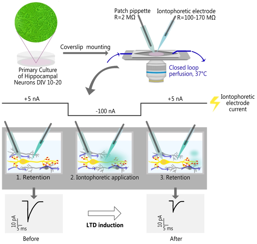
Local iontophoretic application of NMDA, combined with patch-clamp recording of miniature excitatory postsynaptic current (mEPSC) and live-cell fluorescence imaging
Background
Long-term depression (LTD) is an activity-dependent reduction of synaptic strength that is considered to mediate important brain functions such as learning and memory [1–3]. Despite several decades of research, the exact mechanisms of LTD induction and maintenance remain largely elusive. To boost their investigation, easy and reliable methods for eliciting LTD are required. Currently, LTD induction is achieved through either an electrophysiological or pharmacological approach. Both approaches cause a prolonged elevation (lasting up to several hundred seconds) in intracellular free calcium ion concentration ([Ca2+]i), leading to AMPA receptor internalization [3,4]. Electrophysiologically, LTD may be modeled by performing low-frequency stimulation (1 Hz for 200–300 s) of afferent fibers or presynaptic neurons and holding postsynaptic neurons at -40 mV to relieve the Mg2+ block on NMDA receptors (NMDARs) [5–8]. This method requires specialized equipment as well as prior identification of monosynaptically connected neurons, which can be challenging when working with primary cultures. The pharmacological approach to LTD induction is simpler and involves bath application of NMDA (20–50 μM) in the presence of NMDA receptor coactivator glycine (10–20 μM) [6,8–12]. Yet, bath application creates an unpredictable spatio-temporal profile of NMDA concentration and affects all cells in the sample, limiting recordings to a single neuron per sample. To circumvent the drawbacks of previously developed protocols and increase experimental throughput, LTD induction may be accomplished with iontophoresis, a method for rapid and localized drug delivery that is widely used in pharmacological and biophysical studies [13–16]. However, the potential use of iontophoretic application for LTD induction has never been explored.
Here, we provide a detailed protocol of iontophoretic NMDA application for LTD induction in primary cultured hippocampal neurons and describe how it may be coupled with electrophysiological recordings and multicolor epifluorescent imaging. To validate the new protocol, we showed that iontophoretic application of NMDA (100 mM in the electrode) for 1 min produced a long-lasting reduction in the amplitudes of miniature excitatory postsynaptic currents (mEPSCs) and elicited LTD-associated Ca2+-dependent translocation of hippocalcin (HPCA), a neuronal Ca2+ sensor protein, from the cytosol to the neuronal plasma membrane [17,18]. We have also demonstrated that the iontophoresis produced a highly localized concentration gradient, enabling pharmacological targeting of individual neurons. This feature provides a significant advantage over standard bath application, as it allows performing experiments on multiple cells within a single coverslip. This is especially beneficial when working with transfected neurons, given the low success rate of exogenous expression.
It is worth noting that this protocol has great potential for modifications. First, short (up to 10 s) iontophoretic NMDA applications might be used to study various Ca2+-dependent processes. Second, this protocol may be modified to rapidly and locally apply any ionic water-soluble compounds, e.g., glycine or DHPG, to induce long-term potentiation or mGluR-dependent long-term depression of synaptic transmission, respectively [12,19]. Finally, this protocol may be easily combined with advanced microscopy techniques such as confocal [8,12], total internal reflection fluorescence (TIRF) [8–10], and stimulated emission depletion (STED) microscopy [12].
Materials and reagents
Biological materials
1. Primary neuronal culture DIV 10–20 (see [20,21] for hippocampal culture, see [21] for cortical culture)
2. Plasmids for transient transfection: HPCA-EYFP [17], PSD-95-pTagRFP (Addgene #52671)
Note: This protocol does not cover procedures for the cultivation and transient transfection of neurons.
Reagents
1. NaCl (MilliporeSigma, catalog number: S9625)
2. KCl (MilliporeSigma, catalog number: P3911)
3. CaCl2 (MilliporeSigma, catalog number: C3881)
4. MgCl2·6H2O (MilliporeSigma, catalog number: M2670)
5. NaOH (MilliporeSigma, catalog number: S8045)
6. KOH (MilliporeSigma, catalog number: P1767)
7. Methanesulfonic acid (MilliporeSigma, catalog number: 47356)
8. Magnesium ATP (MilliporeSigma, catalog number: A9187)
9. Sodium GTP (MilliporeSigma, catalog number: G8877)
10. Disodium phosphocreatine (MilliporeSigma, catalog number: P7936)
11. EGTA (MilliporeSigma, catalog number: E0396)
12. HEPES (MilliporeSigma, catalog number: H7523)
13. Glucose (MilliporeSigma, catalog number: G7528)
14. Anhydrous DMSO (MilliporeSigma, catalog number: D2650)
15. NMDA (MilliporeSigma, catalog number: M3262)
16. Glycine (MilliporeSigma, catalog number: G7126)
17. Tetrodotoxin citrate (TTX) (Tocris, catalog number: 1069); prepare 5 mM stock solution according to manufacturer protocol
18. Alexa Fluor 594 hydrazide (Thermo Fisher, catalog number: A10438)
19. Fluo-4/AM (Thermo Fisher, catalog number: F14201)
20. Ethanol, 96% v/v
Solutions
1. HEPES buffered saline (HBS) with 1 mM/0.3 mM Mg2+ (see Recipes)
2. KCl-methanesulfonate intracellular solution (see Recipes)
3. HEPES (0.5 M, pH 7.3, stock solution in ddH2O) (see Recipes)
4. NMDA (100 mM, stock solution in 10 mM HEPES, pH 7.3) (see Recipes)
5. Glycine (100 mM, stock solution in 10 mM HEPES, pH 7.3) (see Recipes)
6. Alexa Fluor 594 (5 mM, stock solution in 10 mM HEPES, pH 7.3) (see Recipes)
7. Fluo-4/AM (5 mM, stock solution in DMSO) (see Recipes)
Recipes
A. Extracellular solution
Note: Alternative compositions for an extracellular solution only differ by the concentration of Mg2+, which is crucial for studying NMDAR-dependent signaling, so you could choose only one that is appropriate for the particular experimental design.
1. HEPES buffered saline (HBS) with 1 mM/0.3 mM Mg2+
| Reagent | Final concentration | Quantity or volume |
|---|---|---|
| NaCl | 150 mM | 4,383 mg |
| KCl | 2.5 mM | 92.5 mg |
| CaCl2 | 2 mM | 147 mg |
| MgCl2·6H2O | 1 mM/0.3 mM | 102 mg/30.5 mg |
| HEPES | 10 mM | 1,192 mg |
| ddH2O | n/a | 500 mL |
I = 160 mM, osmolarity ~290–310 mOsm/L.
Notes:
1. Dissolve all components in ~3/4 of the final volume, adjust pH to 7.3 with 2–3 M NaOH solution, and adjust the volume to the final value. Filter and store at 4 °C for no longer than 6 months.
2. Add glucose before the start of the experiment (9 mg per 10 mL of HBS).
B. Intracellular solution
2. KCl-methanesulfonate intracellular solution
| Reagent | Final concentration | Quantity or volume |
|---|---|---|
| KCl | 10 mM | 18.64 mg |
| Methanesulfonic acid | 135 mM | 324.37 mg |
| Magnesium ATP | 4 mM | 50.7 mg |
| Sodium GTP | 0.4 mM | 5.23 mg |
| Disodium phosphocreatine | 5 mM | 31.89 mg |
| EGTA | 0.5 mM | 4.75 mg |
| HEPES | 10 mM | 59.5 mg |
| ddH2O | n/a | 25 mL |
Osmolarity ~270–290 mOsm/L.
Note: Methanesulfonic acid is highly viscous; handle it carefully. The necessary volume is 219 μL (ρ = 1.481 g/mL). Dissolve all components in ~3/4 of the final volume, adjust pH to 7.3 with KOH, and adjust the volume to the final value. Make 0.5 mL aliquots and store at -20 °C for no longer than 12 months.
C. Pharmacological compounds and dyes
3. HEPES (0.5 M, pH 7.3, stock solution in ddH2O)
| Reagent | Final concentration | Quantity or volume |
|---|---|---|
| HEPES | 0.5 M | 2.979 mg |
| ddH2O | n/a | 25 mL |
Note: Dissolve all components in ~3/4 of the final volume, adjust pH to 7.3 with 2–3 M NaOH solution, and adjust the volume to the final value. Filter and store at 4 °C. This stock buffer solution is used to dissolve pharmacological compounds and dyes.
4. NMDA (100 mM, stock solution in 10 mM HEPES, pH 7.3)
| Reagent | Final concentration | Quantity or volume |
|---|---|---|
| NMDA | 100 mM | 7.36 mg |
| HEPES stock solution (Recipe 3) | 10 mM | 10 μL |
| ddH2O | n/a | 490 μL |
Note: Given that it may be difficult to weigh small quantities of NMDA, weigh the compound directly in the 1.5 mL reaction tube, and use the following relationship to estimate the appropriate volume of stock solution components: 66.608 μL of ddH2O and 1.359 μL of 0.5 M HEPES, pH 7.3 per1 mgof NMDA (MW = 147.13 g/mol). Add ddH2O first, then the buffer stock solution; dissolve the compound with active tube agitation or vortexing. Briefly centrifuge the tube to collect all the solution at the bottom, aliquot it, and store at -20 °C for no longer than 6 months.
5. Glycine (100 mM, stock solution in 10 mM HEPES, pH 7.3)
| Reagent | Final concentration | Quantity or volume |
|---|---|---|
| Glycine | 100 mM | 37.55 mg |
| HEPES stock solution (Recipe 3) | 10 mM | 0.1 mL |
| ddH2O | n/a | 4.9 mL |
Note: Add ddH2O first, then the buffer stock solution; dissolve the compound, aliquot it, and store at -20 °C for no longer than 10–12 months.
6. Alexa Fluor 594 (5 mM, stock solution in 10 mM HEPES, pH 7.3)
| Reagent | Final concentration | Quantity or volume |
|---|---|---|
| Alexa Fluor 594 | 5 mM | 1 mg |
| HEPES stock solution (Recipe 3) | 10 mM | 5.27 μL |
| ddH2O | n/a | 258.31 μL |
Note: Volume estimated for 1 mg of dye (MW = 758.79 g/mol); add ddH2O first, then the buffer stock solution, and dissolve the compound by shaking or vortexing. Briefly centrifuge the tube to collect all the solution at the bottom, aliquot it, and store at -20 °C no longer than 10–12 months.
7. Fluo-4/AM (5 mM, stock solution in DMSO)
| Reagent | Final concentration | Quantity or volume |
|---|---|---|
| Fluo-4/AM | 5 mM | 50 μg |
| DMSO | n/a | 9.12 μL |
Note: Volume estimated for 50 μg of dye (MW = 1096.95 g/mol); add DMSO and dissolve the dye with gentle pipetting; use only anhydrous DMSO; the presence of H2O in the solvent may dramatically affect dye solubility. Briefly centrifuge the tube, aliquot the solution, and store at -20 °C for no longer than 10–12 months. Try to reduce the number of freeze-thaw cycles of aliquots and check for the presence of precipitate before using. Pipette the solution if necessary.
Laboratory supplies
1. 35 mm Petri dish (CellStar, catalog number: 627160)
2. 1.5 mL reaction tube (Greiner, catalog number 616 201)
3. Glass capillaries with filament O.D. 1.5 mm, I.D. 0.86 mm (Sutter Instrument, catalog number: BF150-86-10)
4. 2.5 mm box-shaped heating filament for microelectrode puller (Sutter Instruments, catalog number: FB255B)
5. Tygon® tube O.D. 2.4 mm I.D. 0.7 mm (Saint-Gobain, catalog number: B-44-4X)
6. Silicon tubing (VWR, catalog number: 228-0701)
7. Luer to tube assortment kit (WPI, catalog number: 504954)
8. Luer valve assortment kit (WPI, catalog number: 14011)
9. Luer-lock syringes (any available with a volume of 1, 10, and 20 mL)
10. Silicone grease (Warner Instruments, catalog number: W4 64-0275)
11. Cross-locking tweezer (Dumont, catalog number: 0202-N5-PS)
12. MicroFil flexible needle (WPI, catalog number: MF28G67-5)
13. Alcohol burner
Equipment
A. Imaging and electrophysiology
1. Inverted microscope (Olympus, model: IX71)
2. 40× oil-immersion high-aperture objective (Olympus, model: UApo/340 40×/1.35)
3. Optical filters set (suitable for selected fluorophores, in our case, Chroma, model: 69008)
4. Dual-view splitter (Optical Insights, model: MSMI-DV-FC)
5. Digital camera (PCO, model: SensiCam QE)
6. Vibration isolation table (CleanBench, model: TMC)
7. Imaging control unit (TILL Photonics, model: ICU2)
8. Monochromator (TILL Photonics, model: Polychrome V)
9. Patch clamp amplifier (HEKA, model: EPC 10)
10. Micromanipulators (Sutter Instrument, model: MPC-200)
11. Ag/AgCl pellets (WPI, catalog number: EP1)
12. Experimental chamber (Warner Instruments, model: RC-25 or DIY analog)
13. Microelectrode puller (Sutter Instrument, model: P-97)
14. BNC cables
15. Computer for setup control
16. Compact benchtop incubator (any capable of maintaining 37 °C, e.g., VWR, model: INCU-Line IL 10)
B. Gravity-fed perfusion system (optional)
17. Peristaltic pump (Kamoer, model: DIPump550)
18. Flow dial (Bioscience Tools, model: PS-FLOW)
19. Temperature controller (Warner Instruments, model: TC-344B)
20. In-line heater (Warner Instruments, model: SH-27B)
21. Magnetic clamp for outlet tube (Warner Instruments, model: MAG-2)
22. Valve controller (Bioscience Tools, model: cValve-6)
23. Solenoid valves (NResearch Inc., models: 161P021, 161P091)
Note: We validate our protocol in the presence and absence of continuous perfusion, but a closed-loop perfusion system is highly recommended for consistent washout kinetics and reproducibility. See the detailed description of the perfusion system in supplementary Figure S1 and Figure S2; 3D models of perfusion system parts for fused deposition modeling (FDM) printing can be provided upon request.
Software and datasets
A. Experimental setup control
1. PatchMaster (v2x69, HEKA, Germany)
2. Live Acquisition (v2.6.0.12, FEI, Germany)
B. mEPSC analysis
3. Clampfit (v11.3, Molecular Devices, USA)
4. NeuroExpress (v24.8.02, GitHub: github.com/attilaszuc/NeuroExpress-patch-clamp-analysis)
C. Image analysis
5. napari (v0.4.19) [22]
6. domb-napari plugin (v0.3.0) [23]
Procedure
A. Coverslip transfer into the HBS
Note: Long-term cultivation results in slight evaporation of the cultivation medium, even in a humidified incubator environment. This causes changes in the medium's osmolarity. Direct transfer of the cells from the cultivation medium to saline solution can result in osmotic shock, followed by cell detachment and reduced viability. To prevent osmotic shock, we gradually transfer the cells to the saline solution by replacing the culture medium in several steps, with incubation periods between each step.
1. Before starting the procedures, prepare the appropriate HBS solutions with the following additions:
• Glucose to a final concentration of 5 mM (9 mg per 10 mL).
• Glycine to a final concentration of 10 μM (1 μL of 100 mM stock solution per 10 mL).
• TTX to a final concentration of 500 nM (1 μL of 5 mM stock solution per 10 mL).
Prewarm the extracellular solution to 37 °C.
Note: Glycine is a required NMDA receptor coactivator. TTX is necessary for mEPSC recordings and avoiding spontaneous calcium spikes.
Caution: Step A2 is performed in a tissue culture room using a biosafety cabinet.
2. Transfer ~0.5 mL of culture medium from a 12-well plate into the 35 mm Petri dish. Make sure that the coverslip with cells remains fully covered by the remaining medium. Then, transfer the coverslip using tweezers. Finally, transfer the remaining medium.
Critical: Use only HBS prewarmed to 37°C in all following steps, as thermal shock may cause cells to detach from the coverslip.
3. To prevent osmotic shock, gradually replace the culture medium with the HBS according to the volume exchange sequence from Table 1 and incubate at 37 °C. After the last step, replace the whole extracellular solution volume with the HBS. Keep cells at 37 °C in the benchtop incubator.
Table 1. Osmolarity adjustment sequence
| Remove volume | Add volume | Incubation time |
|---|---|---|
| - | 500 μL | 10 min |
| 500 μL | 700 μL | 10 min |
| 700 μL | 1,000 μL | 10 min |
B. Loading the neurons with the cell-permeable Ca2+ indicator Fluo-4/AM
Optional: Skip these steps if Ca2+ imaging is not required; adaptation of the protocol from [24].
1. Prepare 5 μM Fluo-4/AM loading solution: draw 0.5 μL of 5 mM Fluo-4/AM stock solution into a 1.5 mL reaction tube, add 500 μL of HBS, and mix well.
2. Replace the HBS in the Petri dish with Fluo-4/AM loading solution and incubate for 20 min at 37 °C.
3. Discard the loading solution, rinse the cells with 500 μL of HBS once, and replace the entire volume with the new 1 mL HBS. Keep the loaded cells at 37 °C.
C. Mounting the coverslip into an experimental setup
1. Prepare all parts of the experimental chamber (Figure 1A). Apply a thin layer of silicone grease around the glass attachment hole on the chamber platform (top surface) and chamber insert (bottom surface) (indicated with blue circles in Figure 1B).
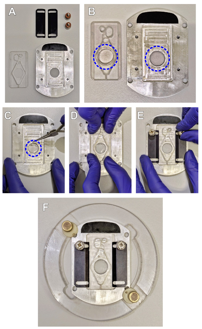
Figure 1. Experimental chamber assembly. (A) Parts of the experimental chamber. (B) Silicone grease application: on the bottom surface of the chamber insert (left), and top surface of the chamber platform (right). (C-E) Installing and securing the coverslip in the experimental chamber. (F) Fully assembled experimental chamber it the microscope stage adapter.
2. Using tweezers, position the glass so that the silicone layer on the chamber platform touches the edge of the glass (Figure 1C, dashed circle indicates the position of the coverslip). Cover the glass with the chamber insert (Figure 1D) and tighten the chamber side clamps (Figure 1E). Add 1 mL of HBS to the chamber and check for any leakage using Kimwipes or a napkin. Gently remove the excess grease from the outer side of the coverslip with an alcohol wipe if necessary (make sure not to smear the grease). Place the assembled chamber in the stage adapter and secure it with the side screws (Figure 1F).
Critical: Try to mount the coverslip as quickly as possible. To prevent the cells from drying out, you may apply a few drops of HBS to the cells after placing the glass on the chamber platform.
3. Apply a drop of immersion oil to the objective lens, place the assembled chamber with the stage adapter in the microscope, and position the reference electrode into the suction reservoir of the chamber (white arrow in Figure 2B). Using transmitted light, focus on the cells and check whether they endured the transfer process.
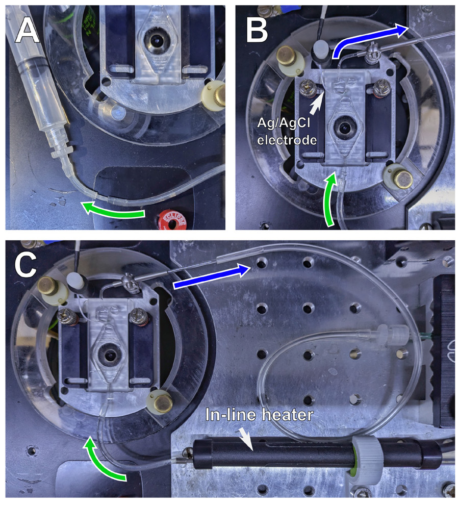
Figure 2. Perfusion setup. (A) Perfusion inlet connector with aspiration syringe for air removal. (B) Experimental chamber with connected perfusion tubes and reference electrode after installation. (C) General view of the experimental chamber setup on the microscope stage. Green: the perfusion inlet connector; blue: the perfusion outlet connector. The white arrow in panel B indicates the reference Ag/AgCl electrode position; the white arrow in panel C indicates the mounted in-line heater connected to the experimental chamber inlet.
4. Set up the perfusion system (see system overview in Figure S2). Close a two-way valve (2 in Figure S2), pour the HBS (10–20 mL) into the main extracellular solution tank (1 in Figure S2), set the flow dial to the "open" position (3 in Figure S2), connect a separate syringe to the perfusion inlet connector tube, open the two-way valve, and aspirate to remove air from the tubing (Figure 2A). Once the tubing is filled with HBS, close the two-way valve.
5. Insert the inlet connector tubing into the imaging chamber inlet port, turn on the peristaltic pump, and position the perfusion outlet so that the tip of the tubing barely touches the solution surface in the suction reservoir (Figure 2B). Then, open the two-way valve and set the input flow to ~2 mL/min (125 mL/h on the flow dial). Adjust the position of the outlet connector to ensure a stable flow through the chamber. Turn on the temperature controller and set it to 37 °C (Figure 2C).
Critical: With continuous perfusion and heating of the extracellular solution, cells remain in optimal condition for up to 2–3 h. However, noticeable bacterial contamination may be observed after 1–1.5 h of perfusion.
Caution: Monitor the meniscus in the imaging chamber carefully; any disruptions in laminar flow reduce perfusion efficiency. Ensure that suction operates in an aspiration regime, i.e., the rate of the outflow should be much higher than the rate of inflow.
D. Fabrication, filling, and positioning of iontophoretic electrode
1. Fabricate several 100–150 MΩ iontophoretic electrodes; see the puller program in Table 2.
Notes:
1. Given that the tips of iontophoretic electrodes are quite thin, we recommend using capillarieswithfilaments to avoid filling issues.
2. During the experimental day, iontophoretic electrodes may become clogged with cell debris; therefore, we recommend fabricating 4–6 electrodes. Store fabricated electrodes in a closed storage box (e.g., Sutter Instruments, catalog number BX10) to avoid clogging with dust.
Table 2. Program for P-97 puller for fabrication of iontophoretic electrodes
| HEAT | PULL | VEL | TIME | PRESSURE |
|---|---|---|---|---|
| Ramp value | 55–60 | 70–80 | 250 | 500 |
2. Thaw an aliquot of 100 mM NMDA stock solution at 4 °C.
Note: Typically, 50–100 μL of NMDA solution is sufficient per experimental day.
3. Fill the iontophoretic electrode with NMDA solution using a MicroFil needle connected to a syringe or directly to a measuring pipette (typically, 10–20 μL of solution is enough).
4. Gently tap the electrode to remove air bubbles and allow the solution to enter the very tip.
5. Insert the electrode into the pipette holder. Make sure that the solution inside the electrode reaches the AgCl probe of the pipette holder. Position the electrode tip above the liquid surface in the chamber (Figure 3Aa). Start PatchMaster software and open Amplifier and Oscilloscope windows.
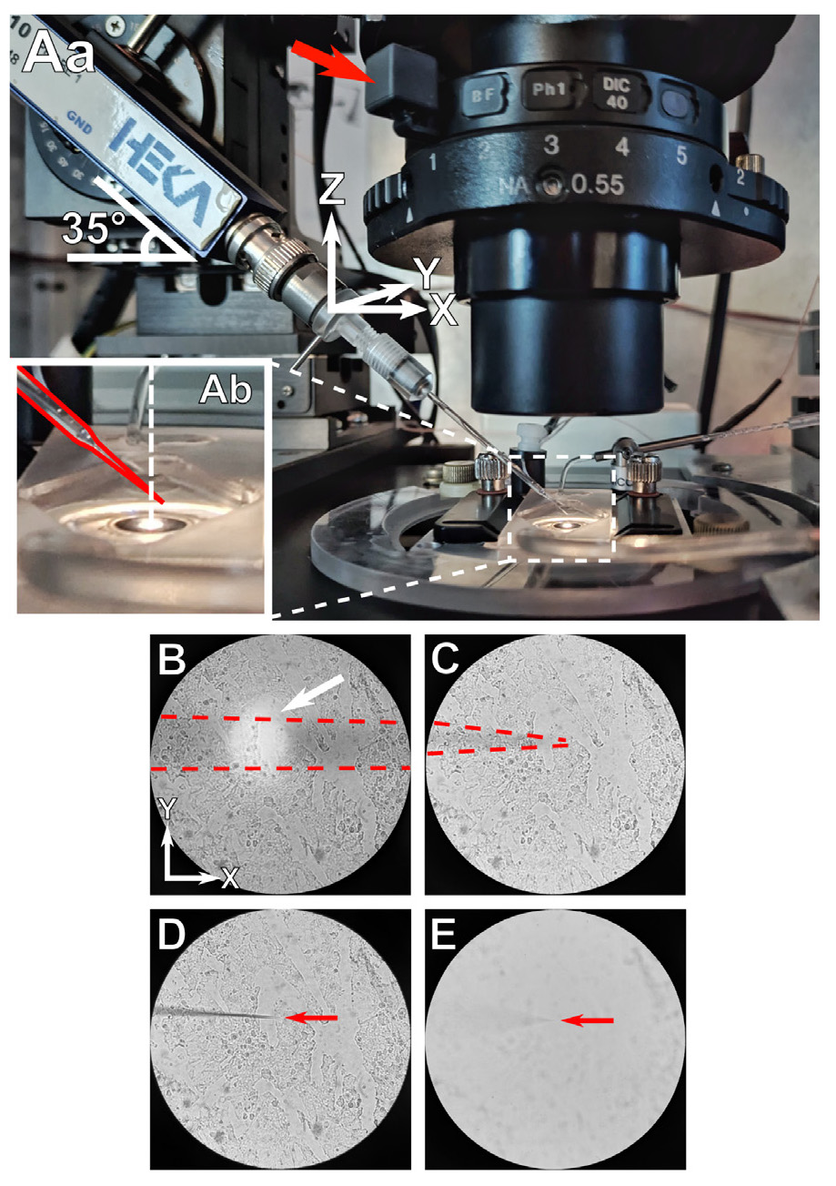
Figure 3. Positioning the iontophoretic electrode. (Aa) General view of the iontophoretic electrode setup on the microscope stage. (Ab) Zoomed in view of the electrode positioned above the experimental chamber before dipping into the solution. Shadow of the electrode shaft (B) and the electrode tip (C) during positioning. Influence of the fully closed (D) and the fully opened (E) condenser diaphragm on the electrode image.
6. Position the iontophoretic electrode inside the chamber and focus on its tip. For that, we recommend the following steps (all directions are given according to our setup with the micromanipulator mounted on the left side):
a. When the electrode is placed above the chamber, ensure that the tip is positioned behind and to the right of the optical axis of the objective (Figure 3Ab; the electrode is highlighted in red, and the white vertical dashed line indicates the optical axis of the objective).
b. Immerse the electrode tip into the chamber solution, checking the resistance. Stop when the initial resistance in the GΩ range jumps down to the electrode resistance of ~100–150 MΩ.
Note: If the electrode resistance exceeds 170–200 MΩ, it is probably clogged and should be replaced. If the problem is repeated with the next electrode, it is recommended to adjust the program of the pipette puller by reducing the HEAT value by 3–5 units.
c. In PatchMaster, press Setup in the amplifier window to reset the recording channel settings, switch to current clamp mode, and set a retention current of +3–6 nA.
Note: The polarity of the retention current is determined by the charge of the pharmacological compound ion in the electrode solution; at pH 7.3, NMDA ions are negatively charged.
Critical: Until the retention current is set, NMDA will flow freely from the electrode and may activate surrounding neurons; therefore, set the retention current as fast as possible.
d. Move the electrode toward yourself (Y-axis) until you come to observe a shadow created by the electrode.
e. Move the electrode to the left along the X-axis while keeping its shadow centered in the field of view. When a bright spot overlaps with this shadow, it indicates where the electrode intersects with the liquid surface (Figure 3B, white arrow).
f. Continue moving the electrode to the left (X-axis) until you reach the end of its shadow (Figure 3C). Then, move the electrode downward along the Z-axis until you focus on the tip (Figure 3F, red arrow indicating electrode tip).
Note: We recommend closing the condenser iris (iris lever marked with a red arrow in Figure 3Aa) to obtain maximum depth of field; Figure 3D shows the field of view with the iris closed, and Figure 3E shows the same field of view with the iris open.
E. Iontophoretic application combined with live-cell imaging
1. Prepare the iontophoresis protocol: in the PatchMaster software, open the Pulse Generator window (in the context menu Windows → Pulse Generator or hotkey F8). Design the iontophoretic protocol. In our experiments, we perform baseline acquisition for 25 s, which is followed by 60 s application of the NMDA, and a subsequent 155 s washout (total protocol duration of 4 min):
a. Enable external triggering in the timing block by selecting Trigger Series (1 in Figure 4).
b. Decrease the sampling frequency to 1 kHz to reduce the acquisition file size (2 in Figure 4).
c. Set up the output channel; in our case, it is Stim-1 (3 in Figure 4).
d. Set up the acquisition channel. Given that the application is performed in current clamp mode, set up Imon-1 (4 in Figure 4).
e. Declare time segments of the protocol: a 25 s baseline segment with retention current set to 5 nA (I-memb), a 60 s application segment with a current of -100 nA, and a washout segment at 5 nA retention current (5 in Figure 4).
f. Check if the Current Clamp mode is selected (6 in Figure 4) and inspect the protocol (drawing window 7 in Figure 4) to make sure it is set up correctly.
g. Execute the protocol (8 in Figure 4). Now, the amplifier is waiting for the external TTL trigger from the imaging control unit.
Note: Set gain to the lower value (0.005 mV/pA) to achieve a maximum application current of -100 nA.
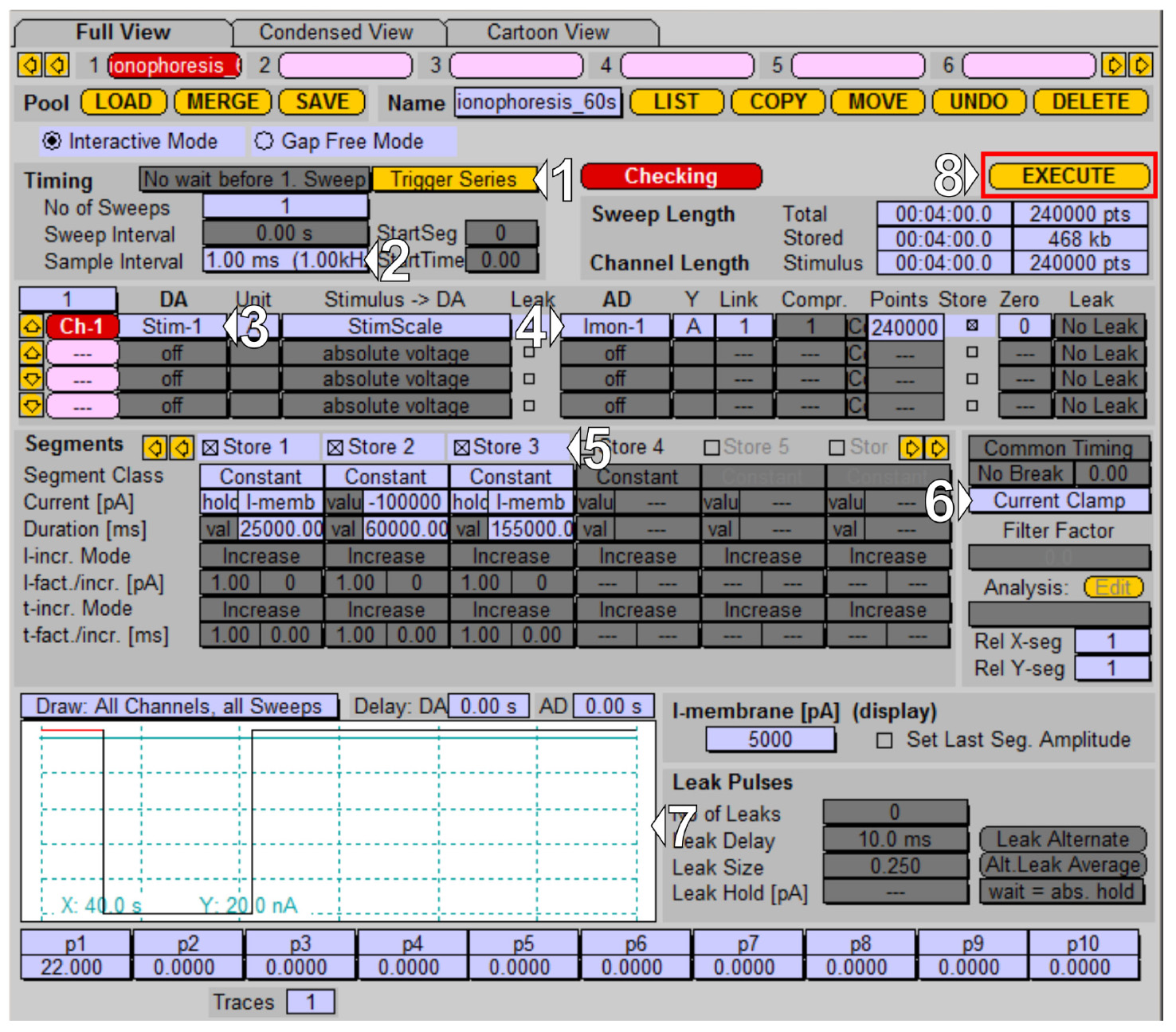
Figure 4. Iontophoretic application protocol managed in the PatchMaster Pulse Generator. (1–4) Triggers and I/O channel settings. (5–7) Application protocol time segments, recording mode, and protocol preview.
2. Start the Live Acquisition software, select the experiment type Multi Channels (1 in Figure 5), select one channel (2 in Figure 5), and set the excitation wavelength (505 nm for EYFP detection in transfected neurons or 495 nm for neurons loaded with the Fluo-4) (3 in Figure 5). To inspect the cells and select a field of view for protocol acquisition, set a few tens of exposure loops (4 in Figure 5), and start the Test Run. Focus on the desired neuron and position it in the center of the field of view.
Note: Keep exposure time to a minimum to reduce photobleaching.
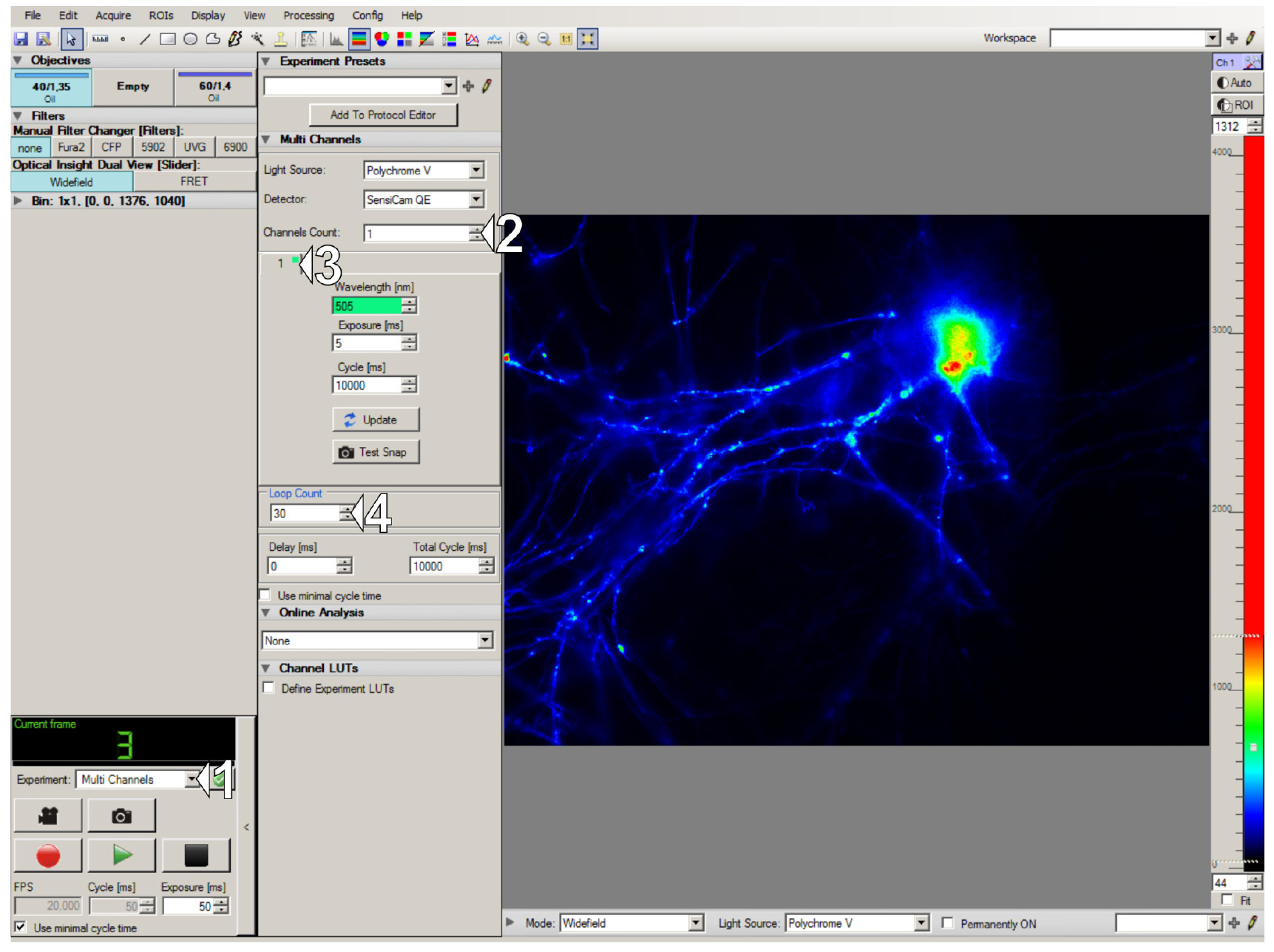
Figure 5. Live Acquisition interface and setting up the test run for choosing a neuron of interest. (1) Experiment type selector. (2-3) Settings of channel number and excitation wavelength. (4) Number of frames for acquisition.
3. Set up Live Acquisition protocol:
a. Select the Protocol Editor experiment type (1 in Figure 6) and add three main items to the protocol: Loop (1×), Trigger (for amplifier triggering), and Multi Channel (6 in Figure 6).
b. (Optional) For dual-channel live-cell imaging of transfected cells: In the Multi Channel tab, select 2 channels and set up excitation wavelengths for both channels: 505 nm for EYFP and 575 nm for TagRFP (2 and 3 in Figure 6).
(Optional) For calcium imaging of cells loaded with the Fluo-4 dye: In the Multi Channel tab, select only 1 channel and set up an excitation wavelength of 495 nm.
c. Set the appropriate Loop Count (48×) and Total Cycle Time (5 seconds), resulting in a total duration of 4 minutes with a frame frequency of 0.2 Hz (4 and 5 in Figure 6).
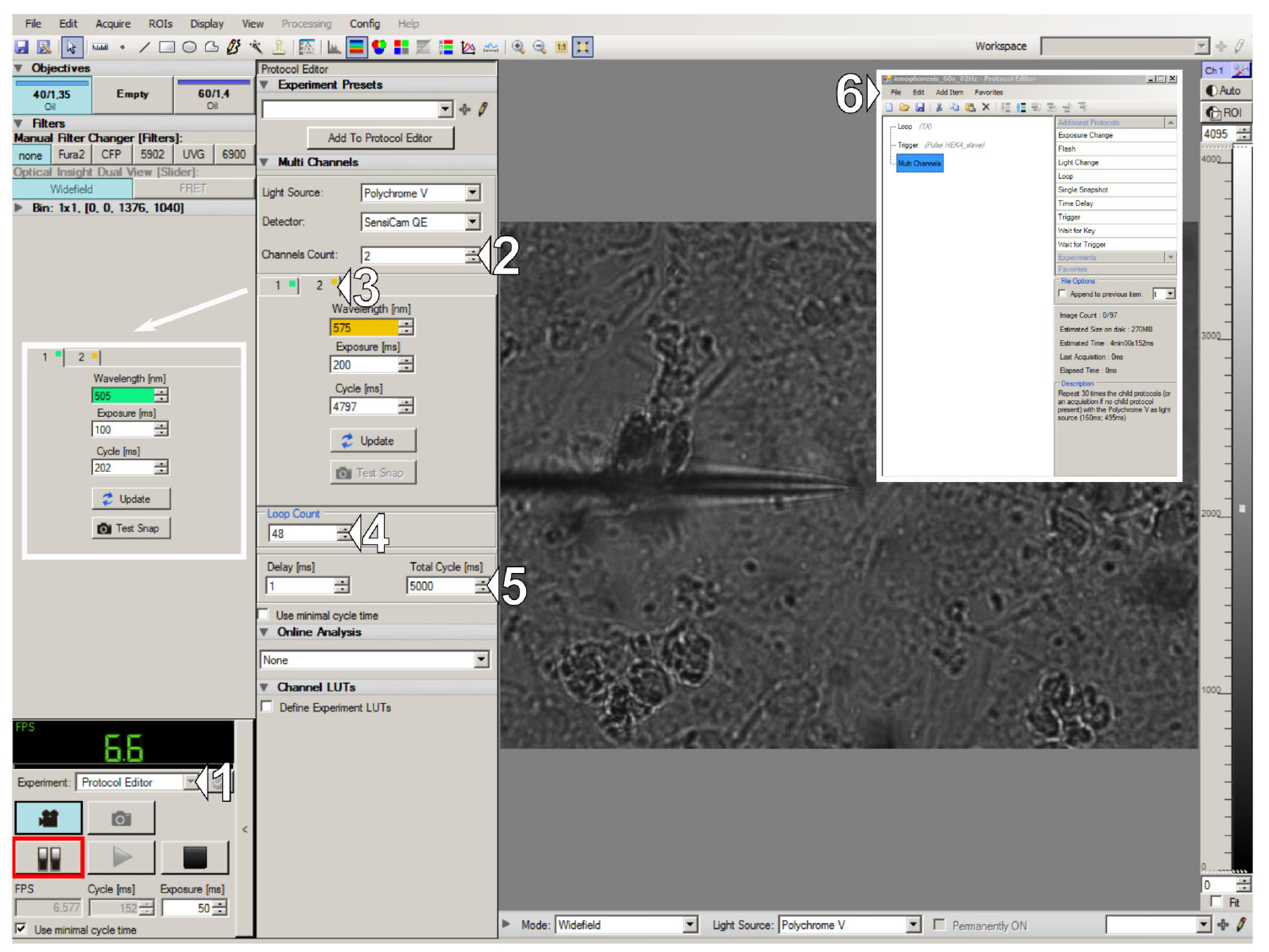
Figure 6. Live Acquisition interface and acquisition protocol design. (1) Experiment type selector. (2) Settings for the number of channels and (3) the excitation wavelength for each channel. (4) Number of frames for acquisition and (5) acquisition frame rate. (6) Acquisition protocol overview.
4. Position the tip of the iontophoretic electrode ~10 μm above the cell of interest.
Note: To increase reproducibility and simplify analysis, position the electrode tip at the exact center of the field of view.
5. Start the protocol acquisition by pressing the Acquire button in Live Acquisition. Monitor the electrode resistance during the protocol; a rapid decrease in current should occur at the beginning of NMDA application. At the end of the application, the current should quickly return to the retention value.
F. Iontophoretic application combined with mEPSCs recordings
Critical: In electrophysiological experiments, induction of NMDAR-LTD requires relieving Mg2+ block on NMDA receptors. To achieve it, iontophoretic application should be accompanied by depolarization of a recorded neuron to -40 mV. Depolarization may be omitted if 0.3 mM Mg2+ HBS is used. It is also possible to use Mg2+-free HBS; however, the absence of Mg2+ in the extracellular solution negatively impacts cell survivability.
1. Prepare the iontophoretic protocol: in the PatchMaster software, open the Pulse Generator window (in the context menu Windows → Pulse Generator or hotkey F8). The protocol includes two independent channels for mEPSC recording and iontophoretic application control, each using separate amplifier headstages:
a. Iontophoretic application: apply a hold current of +5 nA (retention current) for 170 s, deliver an application current of -100 nA for 60 s, and return to a hold value of +5 nA for 320 s.
b. mEPSCs recording: -60 mV holding for 150 s, step to -40 mV holding potential for 100 s (necessary to relieve the Mg2+ block on NMDARs), and return to -60 mV holding potential for 300 s.
2. Choose the desired sampling frequency. To reduce acquisition file size, use 3.33 kHz (sample interval of 300 μs, 1 in Figure 7).
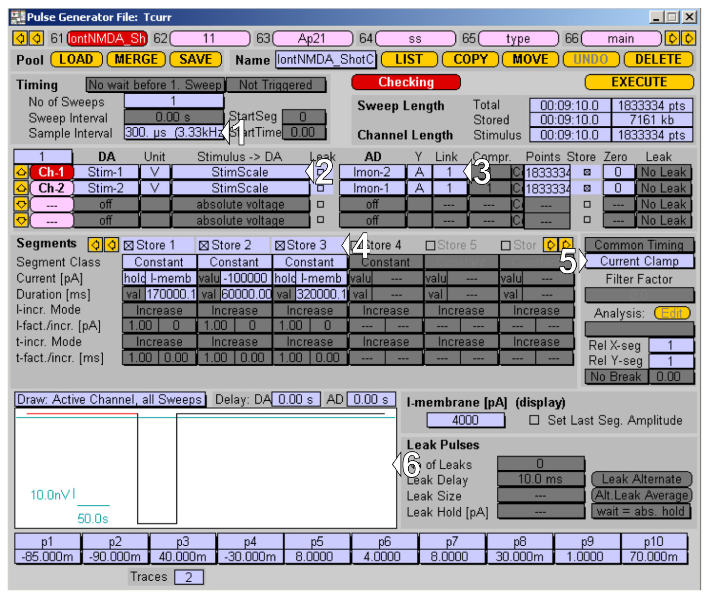
Figure 7. Channel 1 protocol for the iontophoretic application managed in PatchMaster Pulse Generator. (1–3) I/O settings for application channel. (4–6) Application protocol time segments, recording mode, and protocol preview.
3. Create the protocol for Channel 1 for the iontophoretic application:
a. Set up the output channel; in this case, Stim-1 for the iontophoretic electrode (2 in Figure 7).
b. Set up the corresponding acquisition channel for monitoring the application current, setting Imon-1 (3 in Figure 7).
c. Declare time segments of the protocol: baseline segment with holding on retention current (I-memb) for 170 s, application segment with a current of -100 nA for 60 s, and washout segment with retention current (I-memb) for 320 s (4 in Figure 7).
d. Make sure the Current Clamp mode is selected for this channel (5 in Figure 7) and inspect the protocol in a drawing window (6 in Figure 7).
Note: Set gain to the lower value (0.005 mV/pA) to achieve a maximum application current of -100 nA.
4. Create the Channel 2 protocol for mEPSCs recordings:
a. Switch to channel 2 and set up the output channel; in our case, it is Stim-2 for the patch-clamp headstage (1 in Figure 8).
b. Set up the corresponding acquisition channel for mEPSCs recording in voltage-clamp mode, set up Imon-2 (2 in Figure 8).
c. Check whether the Voltage Clamp mode is selected for this channel and activate the Separate Timing option (3 in Figure 8).
d. Declare time segments of the protocol: -60 mV holding for 150 s, depolarization to -40 mV for 100 s, and return to -60 mV holding for 300 s (4 in Figure 8). Inspect the protocol in a drawing window (5 in Figure 8).
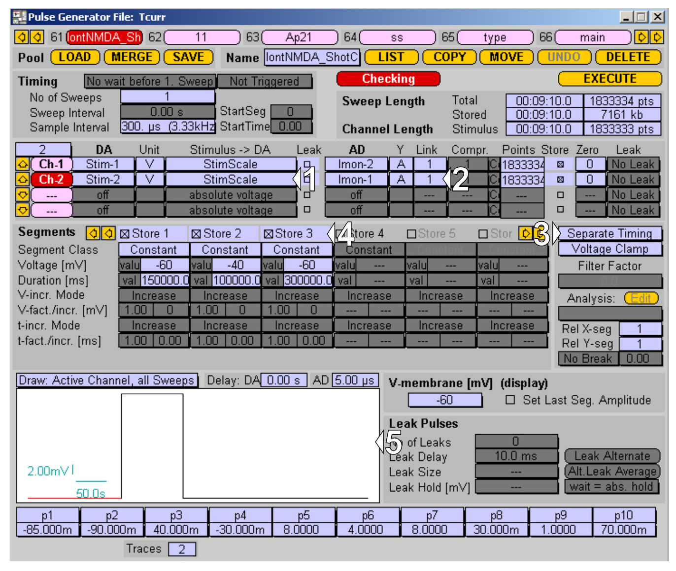
Figure 8. Channel 2 protocol for the mEPSCs recording managed in PatchMaster Pulse Generator. (1–2) I/O settings for recording channel. (4–5) Recording protocol time segments, recording mode, and protocol preview.
5. Using a silicon tube, connect the pipette holder to a two-way Luer valve with an attached mouthpiece (1 mL syringe without the plunger).
6. Thaw a 0.5 mL aliquot of KCl-methanesulfonate intracellular solution, transfer it into a 1 mL syringe, and put on a MicroFil needle.
7. Fabricate several patch pipettes; see the puller program in Table 3. The pipettes should have a resistance of 3-4 MΩ when filled with KCl-methanesulfonate solution.
Table 3. Program for P-97 puller for fabrication of the patch pipette
| HEAT | PULL | VEL | TIME | PRESSURE |
|---|---|---|---|---|
| Ramp value | 0 | 18–25 | 250 | 500 |
8. Fill the patch pipette with KCl-methanesulfonate intracellular solution, insert it into the pipette holder connected to the amplifier headstage, and position the pipette tip above the liquid surface in the chamber.
9. Immerse the pipette tip into the chamber.
10. In the PatchMaster software, press Setup in the amplifier window to reset the recording channel settings. Then, focus on the tip of the patch pipette (the procedure for positioning iontophoretic and patch-clamp pipettes is identical; see step D7 for reference).
11. Visually inspect the pipette opening to ensure it is not obstructed by any debris. Assess pipette resistance and make sure it falls within the 3–4 MΩ range. Using the mouthpiece, apply positive pressure and close the valve to maintain it. Start the Test Pulse in the Amplifier window.
12. Position the pipette above the cell layer: change the focal plane first, then follow up with the pipette. When the pipette is close to the cell layer, switch the manipulator to low speed and position the pipette tip over the center of the target neuron’s soma.
13. Continue descending to the surface of the desired neuron. When resistance begins to increase, monitor it closely. Once the resistance reaches approximately twice the initial value (5–7 MΩ), apply gentle negative pressure using the mouthpiece (similar to sipping through a straw) and close the valve. At this stage, the pipette-reference electrode resistance should rise abruptly. Upon reaching 200–300 MΩ, release the negative pressure. From this point, the gigaseal (the resistance over 1 GΩ), which defines the cell-attached patch clamp configuration, should establish on its own. If that does not happen, facilitate gigaseal formation by switching to negative holding potentials and applying negative pressure with the mouthpiece.
14. Use the C-Fast compensation function to neutralize pipette capacitance. Allow a couple of minutes for cell-pipette contact stabilization. Monitor the baseline current value; ideally, it should be within the 10–20 pA range.
15. Set the holding potential to -60 mV. Then, establish whole-cell patch clamp configuration. For that, apply negative pressure through a mouthpiece and gradually increase it until the cell membrane is ruptured (evidenced by whole-cell capacitive transients in the Oscilloscope replacing the flat test-pulse response). Once the transient appears, release the negative pressure immediately.
16. Compensate cell capacitance with the C-Slow compensation function.
17. Position the iontophoresis electrode ~10 μm above the apical dendrite of the patched neuron.
18. Start the protocol. Monitor the current applied to the iontophoretic electrode; rapid changes should occur at the start and the end of NMDA application (Figure 9, red trace). Monitor the stability of patch clamp recording (Figure 9, black trace). Inspect the series resistance before and after the protocol acquisition, as it tends to increase over time. Ensure that series resistance does not change by more than 20% to prevent compromising the quality of the collected data.
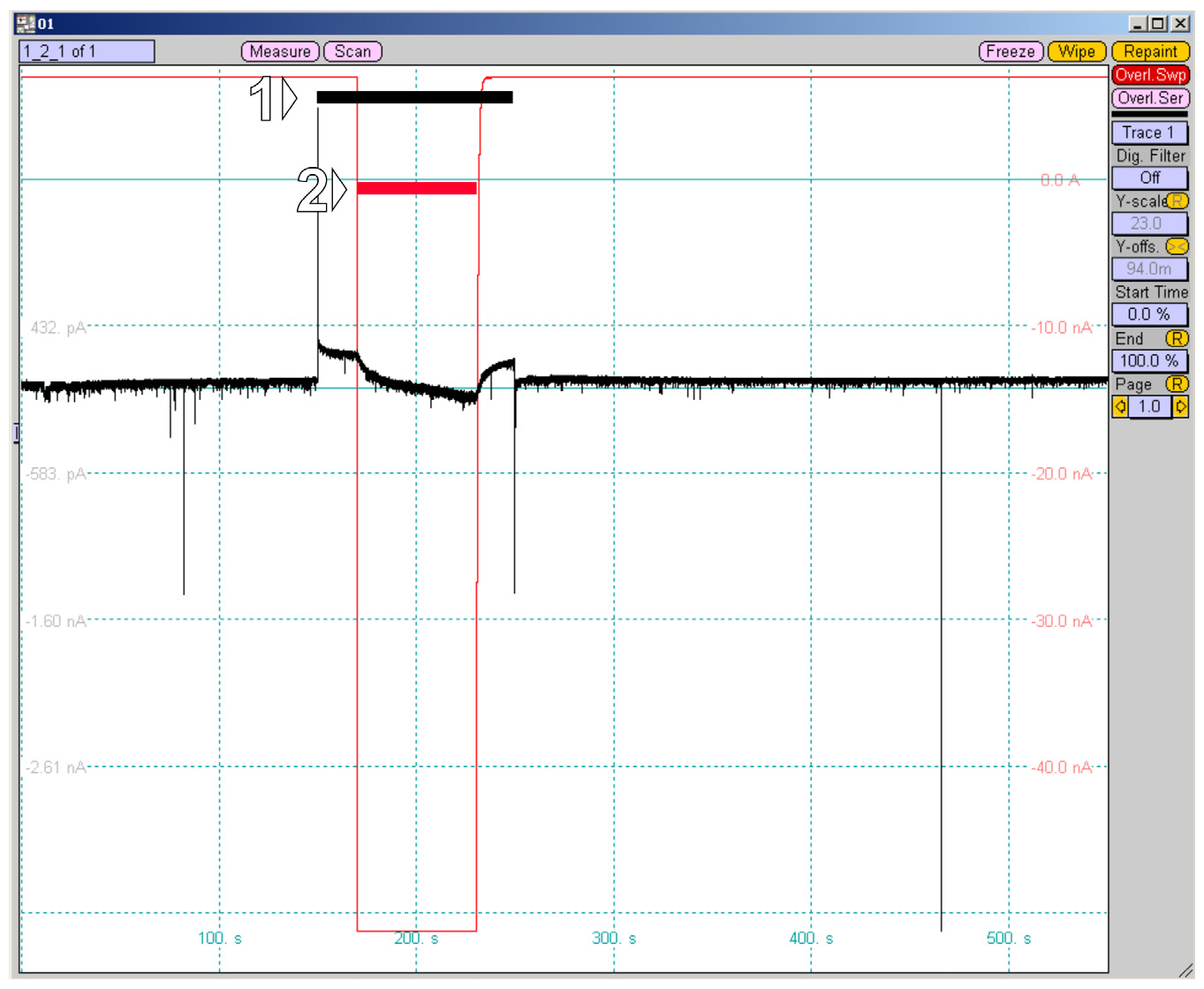
Figure 9. Iontophoretic protocol recorded in PatchMaster Oscilloscope (black, whole-cell recording; red, current on the iontophoretic electrode). (1) Depolarization pulse up to -40 mV for 100 s aimed at relieving the Mg2+ block of NMDARs. (2) Iontophoretic application lasting 60 s.
Data analysis
A. Image analysis
For quick and easy analysis of live-cell imaging data, we developed a specialized plugin for napari, an open-source Python-based viewer for multidimensional images [22], which does not require any programming skills. Below, we provide a brief description of the data analysis pipeline that is used to assess spatial translocation of the neuronal Ca2+ sensor protein HPCA in response to iontophoretic NMDA application (described in Section D of the Procedure). In our example, we use PSD-95-pTagRFP as a fluorescent marker of postsynaptic densities.
Note: To access the comprehensive documentation and report issues on domb-napari plugin, please visit the GitHub repository (github.com/wisstock/domb-napari); all source code is released under the MIT Open Source License. This plugin has been tested for epifluorescent, LSM, and spinning-disk confocal data sets. Currently, the plugin is optimized only for small and medium-sized data. The plugin is not yet optimized for high-throughput acquisitions.
Image analysis pipeline using the domb-napari plugin
1. Preprocessing
The Multichannel stack preprocessing widget provides general image preprocessing functions, including spectral channel splitting to individual images, median filtering, and photobleaching correction with exponential/bi-exponential fitting (Figure 10A). In addition, the Dual-view stack registration widget provides functionality for the affine registration of spectral channels.
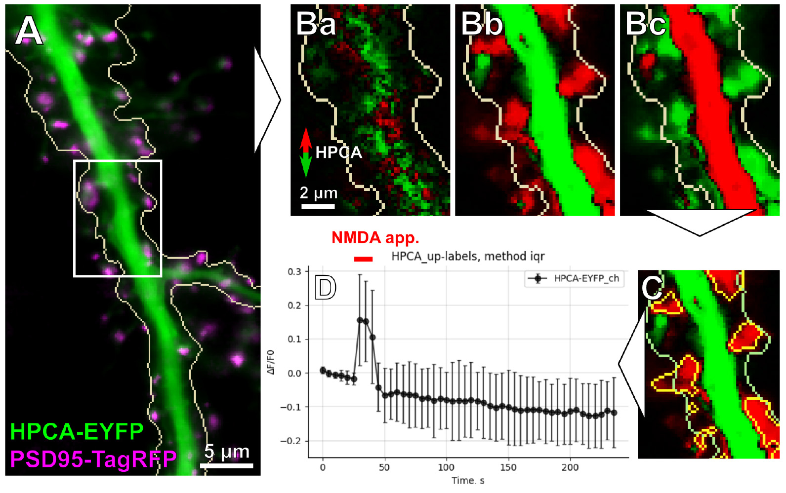
Figure 10. Image analysis pipeline overview. (A) Overlay of the acquired and post-processed HPCA-EYFP and PSD95-TagRFP images of a dendritic tree. The white rectangle indicates the region zoomed in (B) and (C). (B) Differential images (created by the Red-Green Series widget) showing HPCA-EYFP translocation. (Ba) Spatial profile of HPCA-EYFP before the start of iontophoretic NMDA application. (Bb) Maximal HPCA-EYFP redistribution at the onset of NMDA application. Notice that the bulk of the dendritic cytosol (shown in green) is depleted of HPCA-EYFP, which translocates to several sites on the dendritic tree (shown in red). (Bc) Reverse redistribution of HPCA-EYFP to the dendritic cytosol after the termination of NMDA application. (C) Image masks created using the Up Masking widget; yellow masks indicate HPCA-EYFP translocation sites on the dendritic tree. (D) Time-lapse analysis of NMDA-induced HPCA-EYFP insertions into detected regions of interest (ROIs) (the output of the Multiple Labels Stat Profiles widget).
2. Fluorescence redistribution detection
The primary method for detecting the redistribution of fluorescent-labeled targets is a series of differential images. The differential image represents a pixel-by-pixel difference in intensity between an image frame and preceding ones (see our previous work [25] for more details). Red color indicates the zones of increased fluorescence, while green color labels the zones where fluorescence is diminished (Figure 10B). To account for variability in kinetics, the Red-green series widget allows adjusting the time difference between the frames for which the differential image is calculated.
3. Masking
The masking step allows setting up intensity thresholds to label specific regions of interest (ROIs). Intensity-based masking with the Up masking widget may be performed on images of both types, raw fluorescence intensity, and differential images of intensity redistribution. This is particularly useful to detect HPCA translocation sites in full-frame mode (Figure 10C).
4. Exploratory analysis and data frame saving
Fast inspection of intensity changes for any type of mask is available with the ROI profiles widget, which creates averaged intensity profiles for each ROI in a selected mask in absolute (a.u.) or relative change (ΔF/F0) units. The results of the analysis can be saved in CSV format as a tidy data frame of ROI intensities across all frames of an input image. It is also possible to create an aggregate plot of the mean (or median) intensity of all ROIs for a single mask and multiple spectral channels (Multiple images stat profiles widget, Figure 10D) or a single image and multiple masks (Multiple labels stat profiles widget).
B. mEPSCs analysis
Recordings of mEPSCs were analyzed using NeuroExpress software according to the authors' recommendations. Events were detected using the Deviation from baseline algorithm. The amplitudes and inter-event intervals of the detected mEPSCs were subsequently used for statistical analysis.
Note: To convert the HEKA .dat format to the Axon .abf format, we followed the next steps. Export the selected trace from the .dat file as ASCII, multiply all values by 1 × 10¹² to obtain values in pA, and save the modified file with an .atf extension. Then, open the .atf file in Clampfit, set up the sampling frequency and unit type (in our case pA) in the file recovery window, and save as an .abf file.
C. Statistical analysis
All statistical analyses and data visualization were performed using the R language with tidyverse collection [26] and rstatix package [27]. For mEPSCs characteristics comparisons, a Kolmogorov–Smirnov (KS) test was used; for multiple group comparisons, a nonparametric Kruskal–Wallis H-test was used; for all post-hoc pairwise comparisons, a pairwise Wilcoxon test with Benjamini & Hochberg p-value adjustment was used.
Validation of protocol
This protocol or parts of it has been used and validated in the following research article:
• Dovgan et al. (2010). Decoding glutamate receptor activation by the Ca2+ sensor protein hippocalcin in rat hippocampal neurons. Eur J Neurosci. 32(3): 347–358. https://doi.org/10.1111/j.1460-9568.2010.07303.x
A. Characterization of spatio-temporal properties of the iontophoretic application
To characterize the efflux from the electrode tip occurring during iontophoretic application, we loaded the electrode with Alexa Fluor 594 dye (100 μM solution), which, similarly to NMDA, is negatively charged at pH 7.3. The experimental design was the same as for NMDA application: the iontophoretic electrode was placed 10 μm above the cell layer, the perfusion rate was set to 2 mL/min, fluorescence was excited at 570 nm, and data were acquired at 1 Hz.
We found that the distribution of Alexa Fluor 594 (right profile in Figure 11A) was almost symmetrical around the axis of the electrode, indicating that perfusion flow did not considerably skew the gradient of the dye. At the same time, the distribution of intensity around the axis perpendicular to the electrode was asymmetric (top profile in Figure 11A). However, this effect was rather caused by an out-of-focus signal from the dye within the electrode and not by the skewness of the concentration gradient itself. Iontophoretic application was highly localized, given the rapid decrease of the dye concentration with distance: the maximum amplitude of fluorescence intensity was 4-fold lower at 50–70 μm from the tip than in its vicinity (Figure 11B–D). During iontophoretic application, the intensity of Alexa Fluor 594 fluorescence displayed a logarithmic increase, which was followed by an exponential decay once the application was terminated (Figure 11C).
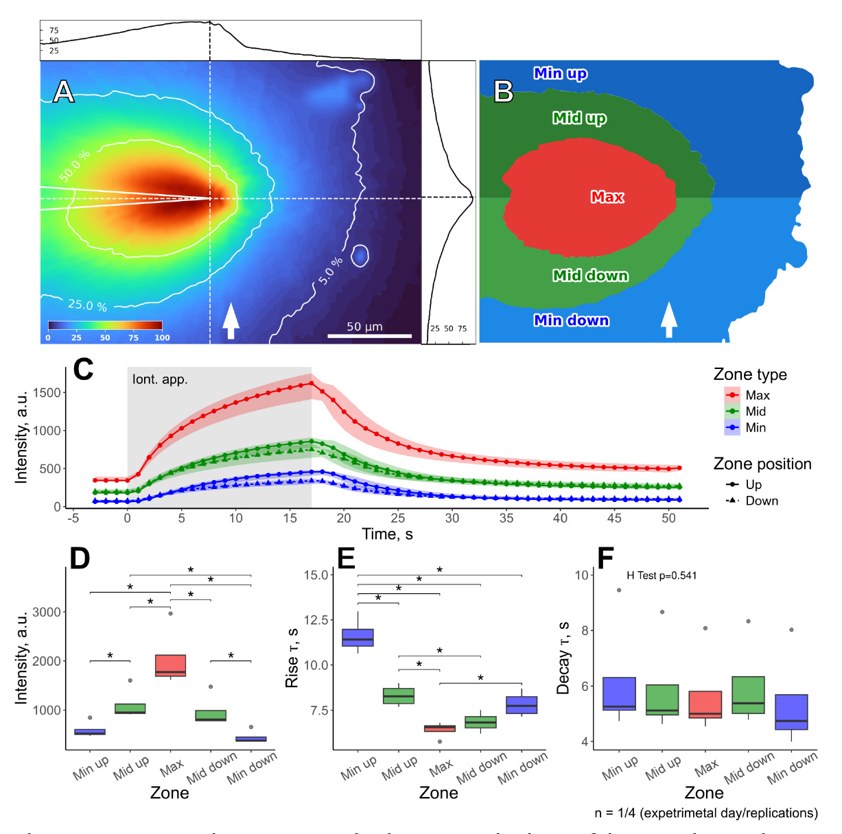
Figure 11. Spatio-temporal characteristics of iontophoretic application assessed with Alexa Fluor 594 dye. (A) Alexa Fluor 594 distribution at the end of iontophoretic application. Colors represent the normalized intensity of fluorescence; contour lines correspond to 50%, 25%, and 5% of maximum intensity. The top and left profiles represent intensity values along the dashed lines intersecting at the electrode tip. The white arrow indicates the direction of the perfusion flow. (B) Image mask showing the distribution zones of Alexa Fluor 594 across the field of view. (C) Time courses of the changes in average intensity of fluorescence for different zones before, during (shaded rectangle) and after iontophoretic application. (D) Maximal intensities of fluorescence for different zones at the end of the iontophoretic application. (E, F) Intensity rise and decay kinetics (time constants of exponential fit) for different zones. *p<0.05, pairwise Wilcoxon test with Benjamini & Hochberg p-value adjustment.
The kinetic properties of the application were rapid (Figure 11E, F): the rise time constant ranged within 5–12 s, while the decay constant was within 4–7 s. As expected, the rise time was fastest in the zone around the electrode tip and decreased with distance (Figure 11E). The rise time values were lower for the zones upstream of the perfusion flow than for the zones downstream of the flow. This suggested that perfusion slightly dispersed the iontophoretic solution along the direction of the flow but did not prevent the diffusion in the opposite direction. Meanwhile, the decay time constant did not vary much across the field of view (Figure 11F), indicating that the washout of iontophoretic solution depended solely on dye diffusion and the rate of perfusion. Overall, iontophoretic application exhibited rapid onset and washout kinetics and created a localized concentration gradient, which was mainly symmetrical to the tip of the application electrode and was not substantially hindered by the active perfusion.
We also investigated appropriate values of retention and application currents using Alexa Fluor 594. We examined the current dependency of the Alexa Fluor 594 response over a wide range of application currents (-25 to -100 nA) and observed no significant differences (see Figure S3); only slight trends were evident. Therefore, for further experiments, we decided to set the application current to the highest value sustained by the amplifier (in our case, -100 nA) to minimize the rise time of the outflow of iontophoretic solution. As for the retention current, we observed a leakage of the fluorescent dye when the values were set to below +1–2 nA. At the same time, high values of retention current (above +10 nA) resulted in a long and inconsistent latency period between switching to the application current and the beginning of the Alexa Fluor 594 outflow from the iontophoretic electrode (data not shown). Hence, in our further experiments, the retention current value was set to +5 nA.
B. Changes in intracellular Ca2+concentration in response to prolonged iontophoretic NMDA application
Next, we characterized [Ca2+]i increase in response to the NMDA application. For that, we loaded neurons with the Fluo-4/AM membrane-permeable Ca2+ indicator (see Procedure, Section B), which was excited at 495 nm. Images were acquired at 1 Hz. The iontophoretic electrode was positioned 30–50 μm from the soma and 10 μm above the apical dendrite. The recording protocol was as follows: (i) a 5 s baseline, the retention current was set to +5 nA to prevent NMDA leakage from iontophoretic electrode, (ii) a 20 s iontophoretic application with the current set to -100 nA, and (iii) NMDA washout for 35 s with retention current at +5 nA.
Given that NMDA receptors are saturated with ~1 mM of NMDA [28], for these experiments, we used a 15 mM NMDA iontophoretic solution to create a saturating concentration gradient across the entire field of view. In our experiments, NMDA treatment induced Ca2+ entry across the dendritic tree in the field of view (Figure 12A, B). However, the spatio-temporal characteristics of [Ca2+]i transients did not strictly coincide with those of iontophoretic application (Figure 12C–E). Despite variance, neither relative changes in Fluo-4 fluorescence intensity (Figure 12D) nor the rise time constants (Figure 12E) showed significant differences between proximal and distant zones in relation to the tip of the iontophoretic electrode. This fact indicates that [Ca2+]i transients depend more on the heterogeneity of dendritic tree morphology, the spatial distribution of NMDARs, Ca2+-stores, and/or dendritic spines than on the NMDA concentration gradient created by iontophoretic application.
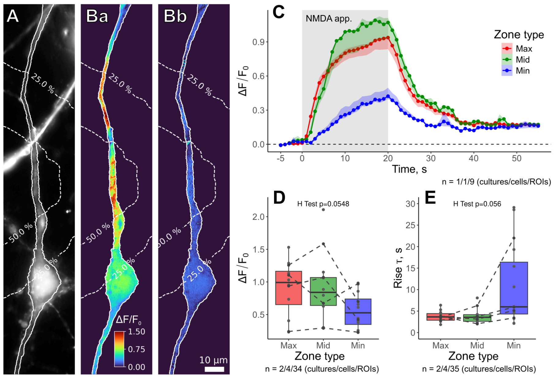
Figure 12. Spatio-temporal characteristics of [Ca2+]i changes induced by iontophoretic NMDA application. (A) Fluorescent image of the tested neuron loaded with the Fluo-4/AM membrane-permeable Ca2+ indicator. Dashed lines represent intensity contour lines from Figure 11A. (Ba) Relative changes of Fluo-4 fluorescence intensity (ΔF/F0) at the end of NMDA application. (Bb) relative fluorescence changes at the end of recording. (C) Time courses of relative fluorescence changes during the NMDA application (shaded rectangle) in different zones. (D, E) Statistical comparisons of maximal relative fluorescence intensities (D) and the rise times (E, time constant of the exponential fit) between the zones at the end of the application.
C. Long-lasting changes in mEPSC properties in response to the iontophoretic NMDA application
To confirm that prolonged iontophoretic NMDA application induced long-term synaptic plasticity, we performed electrophysiological recordings of miniature excitatory postsynaptic currents (mEPSCs). Given that these experiments were conducted using 1 mM of Mg2+ in the extracellular solution, the iontophoretic application was accompanied by depolarization of the neuron to the holding potential of -40 mV to relieve Mg2+ block of NMDA receptors (see Procedure, Section D). For analysis and comparison, the characteristics of detected mEPSCs were averaged over 75 s time intervals, as illustrated in Figure 13A.
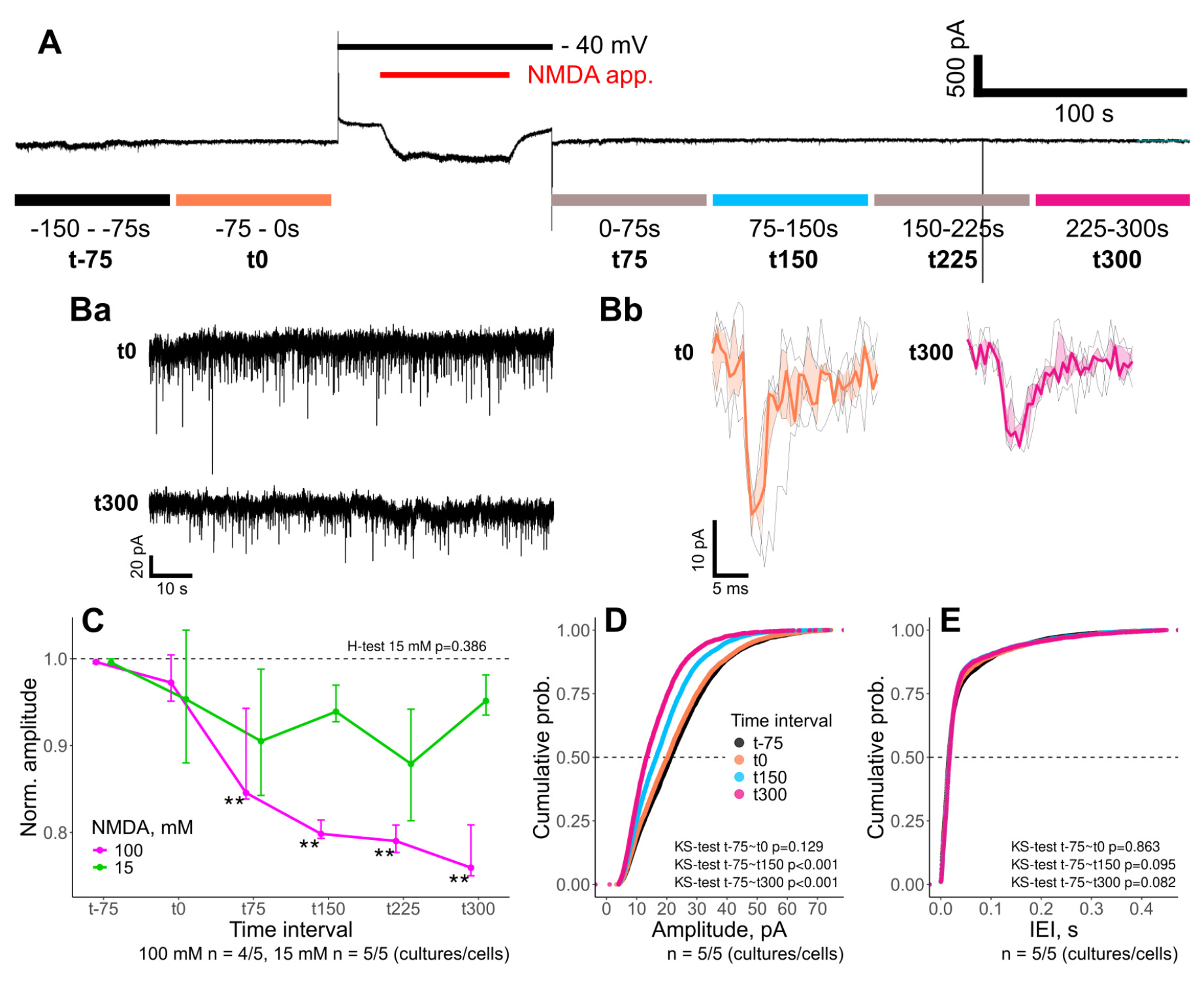
Figure 13. Long-term depression induced by iontophoretic application of NMDA. (A) Representative whole-cell recording showing the iontophoretic application of 100 mM NMDA (red bar on top). Time intervals used for further analysis (color bars on bottom). Representative mEPSCs recording (Ba) and averaged mEPSC (Bb) for selected time intervals. (C) Normalized mEPSC amplitudes for declared time intervals in experiments with 15 mM (green) and 100 mM (magenta) of NMDA in the iontophoretic electrodes. Notice a ~25% decrease in mEPSC amplitudes after 100 mM NMDA application. (D, E) Cumulative histograms of mEPSC amplitudes (D) and inter-event intervals (E) for selected time intervals in experiments with 100 mM NMDA in the iontophoretic electrode. **p<0.01, pairwise Wilcoxon test with Benjamini & Hochberg p-value adjustment.
Given that robust [Ca2+]i transients were observed in response to 15 mM iontophoretic NMDA application (see Validation, Section B), we assumed it would also be able to induce long-term depression. However, application of the 15 mM NMDA solution produced inconsistent changes in mEPSC amplitudes. Likely, the concentration gradient created by the 15 mM NMDA application was too localized and failed to modulate the substantial pool of synapses on the dendritic tree of the studied neuron, affecting only its minor population. Hence, the combined activity of intact (major pool) and modulated (minor pool) synapses contributed to the observed mEPSCs. Meanwhile, application with 100 mM NMDA in the electrode solution reliably induced a significant reduction in mEPSC amplitudes (Figure 13B–D). Comparison of the normalized mEPSC amplitudes between the initial baseline (t-75) and the intervals after 100 mM NMDA application showed a sustained ~25% decrease of mEPSC amplitudes (Figure 13C). Since inter-event intervals of mEPSCs were not altered (Figure 13E), diminished mEPSC amplitudes clearly pointed to the induction of NMDA-dependent long-term synaptic depression.
Therefore, iontophoretic application of 100 mM NMDA for 60 s is an effective approach for the induction of chemLTD at the level of a single neuron. At the same time, iontophoretic solutions with lower NMDA content may still be used to induce LTD in specific subpopulations of synapses.
D. Translocation of neuronal Ca2+ sensor protein HPCA in response to LTD-inducing iontophoretic NMDA application
Given the HPCA involvement in LTD-associated Ca2+-dependent endocytosis of AMPA receptors [18], we sought to confirm HPCA translocation from the cytosol into the cell membranes in response to LTD-inducing iontophoretic NMDA application (100 mM NMDA for 60 s). To detect HPCA insertion into the plasma membrane, a Förster resonance energy transfer (FRET) imaging technique was used. We monitored the energy transfer between ECFP-conjugated HPCA (HPCA-ECFP, donor) and membrane-bound EYFP (EYFP-Memb, acceptor), a nonspecific membrane tag [29]. Since FRET required the distance between donor and acceptor fluorophores to be approximately 100 Å, an increase in FRET suggested the insertion of HPCA-ECFP into the cell membranes [30]. In our experiments, we used a three-cube approach to capture fluorescence of the acceptor elicited by the excitation of the donor [31,32] and quantitatively evaluated FRET efficiency (Eapp) to assess HPCA translocation to the membranes.
We found that LTD-inducing iontophoretic NMDA application significantly altered the Eapp (Figure 14Aa, b). Its changes could be easily identified on the differential images (Figure 14Ab). Time-course data (Figure 14B) showed that the onset of iontophoretic NMDA application elicited a rapid 20%–50% rise in Eapp values, which was followed by a plateau phase throughout the rest of the application. Eapp values slowly recovered after the application was terminated (Figure 14B), indicating HPCA redistribution back to the cytosol. Relative changes in FRET efficiency (ΔEapp/Eapp0) exhibited similar changes (Figure 14C, D). These results confirm transient HPCA translocation to the cell membranes occurring during LTD induction.
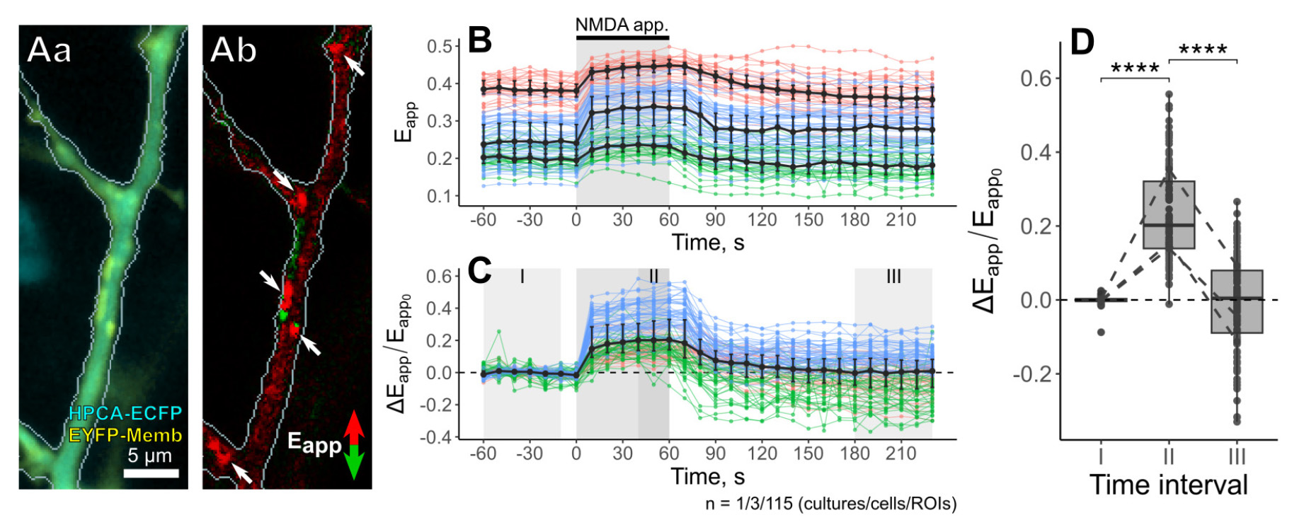
Figure 14. Neuronal Ca2+ sensor protein HPCA translocation in response to LTD-inducing iontophoretic NMDA application. (Aa) Overlay of fluorescent signals from HPCA-ECFP and the membrane tag EYFP-Memb, and (Ab) differential image of FRET efficiency (Eapp) changes in response to iontophoretic NMDA application. White arrows point at the HPCA translocation sites characterized by the highest FRET efficiency (Eapp). (B, C) Time courses of absolute (B) and relative changes (C) in FRET efficiency (Eapp) during 60 s NMDA application (shaded rectangle) for three representative neurons. (D) Comparison of relative Eapp changes before (I), during (II), and after (III) the iontophoretic NMDA application. ****p<0.0001, pairwise Wilcoxon test with Benjamini & Hochberg p-value adjustment.
E. Translocation of HPCA in response to short iontophoretic NMDA application
Finally, we wanted to show that iontophoretic applications could also be useful for investigating LTD-independent HPCA translocation. For that, we repeatedly performed short iontophoretic applications of 100 mM NMDA with decreasing durations (5, 2.5, and 0.5 s). For all tested durations, we observed robust HPCA translocation along the dendritic tree, indicating HPCA insertions into the cell membranes (Figure 15Aa). After NMDA applications were terminated, HPCA left the insertion sites and redistributed back to the cytosol (Figure 15Ab). Sites of HPCA insertion were saturated at 2.5 s NMDA application; neither additional translocation sites nor increased value of HPCA insertion were detected for longer (5 s) applications (Figure 15B, C). HPCA insertions were fully reversed within 10 s after the end of iontophoretic application (Figure 15B), indicating that a relatively short washout period (1–2 min) was required for sequential iontophoretic applications. These facts confirmed that repeating NMDA iontophoretic applications were a suitable approach for studying Ca2+-dependent translocation of neuronal sensor proteins such as HPCA.
To conclude, prolonged iontophoretic application is a practical tool for investigating long-term synaptic plasticity in primary cultured neurons. The iontophoretic application produces a highly localized concentration gradient. This feature reduces the use of pharmacological compounds (compared to the standard bath application) and allows inducing synaptic plasticity in individual neurons on the same coverslip. The latter is particularly convenient for working with transfected cells, given that the transfection rate is usually quite low for neurons. Furthermore, short iontophoretic NMDA applications might also be used to investigate Ca2+-dependent processes such as HPCA translocation.
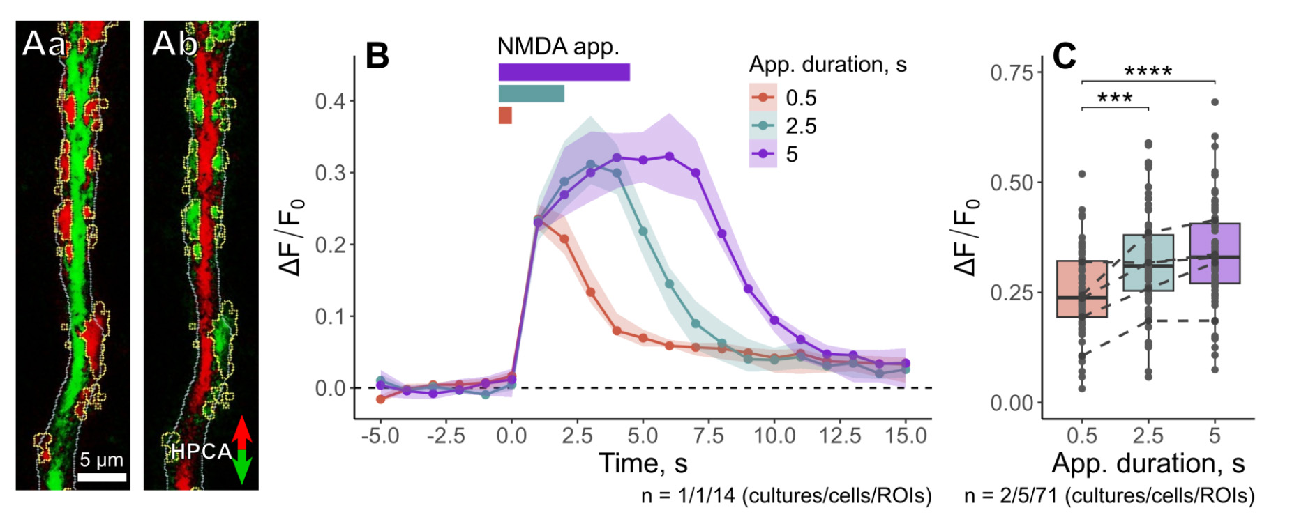
Figure 15. HPCA translocation in response to short iontophoretic NMDA applications. (A) Differential images showing NMDA-induced HPCA translocation. (Aa) Maximal redistribution of HPCA at the onset of the application; HPCA accumulation at specific sites on the dendritic tree is highlighted in yellow. (Ab) Reverse redistribution of HPCA after the termination of NMDA application. (B) Time courses of relative fluorescence changes (ΔF/F0) observed for the same neuron in response to a series of NMDA applications with decreasing durations. (C) Comparison of maximal amplitudes of HPCA translocation for different durations of NMDA application. ***p<0.001, ****p<0.0001, pairwise Wilcoxon test with Benjamini & Hochberg p-value adjustment.
General notes and troubleshooting
General notes
1. Iontophoretic application is a practical tool for delivering pharmacological agents in studies involving primary cultured neurons. Unlike bath application, iontophoresis produces a highly localized concentration gradient, enabling pharmacological targeting of individual neurons. This feature allows performing experiments on multiple cells within a single coverslip, which is particularly convenient for working with transfected neurons, given that the success rate of exogenous expression is usually quite low. Iontophoresis also offers greater versatility compared to a standard bath application. For instance, prolonged iontophoresis using high NMDA concentration in the electrode induces long-term depression in a targeted neuron. At the same time, shorter duration of application and/or lower NMDA content in the electrode still produce robust [Ca2+]i transients, allowing investigation of Ca2+-dependent processes such as translocation of neuronal Ca2+ sensor proteins. Both these approaches might be used in a single experimental protocol. Alternatively, adjusting the duration of application and/or NMDA content in the application electrode may provide an opportunity to alter synaptic transmission within a specific subset of synapses on a dendritic tree.
2. Given that iontophoretic application is suitable for delivering any ionic water-soluble compound, this protocol may be modified to apply glycine or DHPG to induce long-term potentiation or mGluR-dependent long-term depression of synaptic transmission, respectively [12,19].
3. This protocol is fully compatible with any imaging setup that uses open-top imaging chambers. Therefore, iontophoresis could replace bath applications in experimental designs employing advanced microscopy techniques that are widely used in synaptic plasticity research. These include confocal microscopy [8,12], total internal reflection fluorescence (TIRF) microscopy [8–10], and stimulated emission depletion (STED) microscopy [12]. These methods might be particularly beneficial for understanding the exact translocation sites of neuronal Ca2+ sensor proteins.
4. Due to the complexity and multimodality of the described protocol, we highly recommend practicing different steps of the procedure separately before trying to implement the whole protocol at once. 1) Practice mounting the coverslip onto the experimental chamber using a dummy glass. Ensure this process does not take longer than 20–30 s. 2) Practice focusing on the tip of an electrode using a high-magnification, high-aperture objective. This process should not take longer than 1 min. 3) Practice positioning an iontophoretic electrode and a patch pipette in the same field of view without damaging either of them. Practice replacing the patch pipette without disturbing the iontophoretic electrode. 4) Practice patch clamp recordings, focusing on seal stability. 5) Practice single-channel imaging. Figure out excitation wavelengths and exposure times appropriate for your set of fluorophores. Once you are confident with each of these steps, you may start combining them.
Troubleshooting
Steps A5–8
Problem 1: The chamber leaks.
Possible causes: 1) Insufficient silicone grease layer between the glass and the chamber. 2) Glass remains or dust.
Solutions: 1) Apply a layer of silicone between the chamber hole (from the glass side) and between the mounting plate and the glass. Check that you have applied a sufficient layer of silicone before placing the cells with the solution in the microscope. 2) Clean the surface and reapply the grease.
Problem 2: Unable to focus on cells with high N.A. objective.
Possible causes: 1) Objective touches the chamber. 2) Two coverslips are stuck together.
Solutions: 1) Move to the center of the coverslip. 2) Separate the two coverslips and take only one for the experiment.
Problem 3: The cell layer peels off after mounting the coverslip.
Possible cause: Careless removal of the glass with tweezers can result in a torn-off cell layer.
Solution: Carefully transfer the cells with the tweezers without touching the cell growth zone, trying to hold the coverslip by the edge of the glass.
Problem 4: Poor quality of cells/dead cells after coverslip mounting.
Possible cause: Long exposure to air while mounting the coverslip or low temperature of the HBS solution.
Solution: Cells are sensitive to environmental changes and must be transferred quickly and into the prewarmed medium.
Problem 5: Perfusion issues, bad HBS flow.
Possible cause: Poor maintenance of the perfusion system. Bacterial overgrowth.
Solution: After each recorded coverslip, rinse the perfusion system with ~30 mL of distilled water. Then, fill the system with fresh HBS.
Steps B1–7
Problem 6: Broken electrode
Possible cause: Incorrect electrode positioning.
Solution: When searching for an electrode in the field of view, focus 10–20 μm above the cells (z-axis) to prevent the electrode from touching the glass.
Problem 7: The electrode resistance is out of the 200–250 MΩ range.
Possible causes: 1) Inappropriate puller settings. 2) Air or debris clogging the tip of the electrode.
Solutions: 1) Adjust the Heat value. Increase the value to increase the resistance of the tip and vice versa. 2) If debris or air is trapped in the electrode tip, replace the electrode.
Problem 8: The iontophoretic drug does not flow from the electrode during the first application or comes out in small amounts.
Possible cause: The electrode tip is not properly filled.
Solution: Move the electrode away from the cells and apply -100 nA current for 2–3 s to fill the tip.
Supplementary information
The following supporting information can be downloaded here:
1. Figure S1. Piping diagram of the perfusion system
2. Figure S2. Perfusion system setup
3. Figure S3. Spatio-temporal characteristics of iontophoretic application at the different current values of -25, -50, -75, and -100 nA.
Acknowledgments
This protocol was used in [33].
This work was funded by the long-term program of support of the Ukrainian research teams at the Polish Academy of Sciences carried out in collaboration with the U.S. National Academy of Sciences with the financial support of external partners (PAN.BFB.S.BWZ.405.022.2023), National Science Center grant Miniatura (NCN 2023/07/X/NZ1/01669), the Ministry of Education and Science of Ukraine grant (0123U102767), and the National Academy of Science of Ukraine grant (0124U001556).
We are deeply grateful to our colleagues from the YPBiotech, R&D department of the YURiA-PHARM pharmaceutical group of companies, and the Head of YPBiotech, Mr. Oleksandr Hubar, biotechnologist Mr. Nazarii Hrubiian, and junior biotechnologist Ms. Anastasiia Romanenko for the design and assembly of the HPCA-mBaoJin plasmid vector.
Competing interests
The authors declare no other conflicts of interest.
Ethical considerations
Animals were used in accordance with the European Commission Directive (86/609/EEC).
References
- Liu, X., Gu, Q. H., Duan, K. and Li, Z. (2014). NMDA Receptor-Dependent LTD Is Required for Consolidation But Not Acquisition of Fear Memory. J Neurosci. 34(26): 8741–8748. https://doi.org/10.1523/jneurosci.2752-13.2014
- Lisman, J. (2017). Glutamatergic synapses are structurally and biochemically complex because of multiple plasticity processes: long-term potentiation, long-term depression, short-term potentiation and scaling. Philos Trans R Soc Lond B Biol Sci. 372(1715): 20160260. https://doi.org/10.1098/rstb.2016.0260
- Kennedy, M. B. (2013). Synaptic Signaling in Learning and Memory. Cold Spring Harbor Perspect Biol. 8(2): a016824. https://doi.org/10.1101/cshperspect.a016824
- Maynard, S. A., Ranft, J. and Triller, A. (2022). Quantifying postsynaptic receptor dynamics: insights into synaptic function. Nat Rev Neurosci. 24(1): 4–22. https://doi.org/10.1038/s41583-022-00647-9
- Thiels, E., Xie, X., Yeckel, M. F., Barrionuevo, G. and Berger, T. W. (1996). NMDA Receptor-dependent LTD in different subfields of hippocampus in vivo and in vitro. Hippocampus. 6(1): 43–51. https://doi.org/10.1002/(sici)1098-1063(1996)6:1<43::aid-hipo8>3.0.co;2-8
- Wong, J. M. and Gray, J. A. (2018). Long-Term Depression Is Independent of GluN2 Subunit Composition. J Neurosci. 38(19): 4462–4470. https://doi.org/10.1523/jneurosci.0394-18.2018
- Dore, K. and Malinow, R. (2021). Elevated PSD-95 Blocks Ion-flux Independent LTD: A Potential New Role for PSD-95 in Synaptic Plasticity. Neuroscience. 456: 43–49. https://doi.org/10.1016/j.neuroscience.2020.02.020
- Azarnia Tehran, D., Kochlamazashvili, G., Pampaloni, N. P., Sposini, S., Shergill, J. K., Lehmann, M., Pashkova, N., Schmidt, C., Löwe, D., Napieczynska, H., et al. (2022). Selective endocytosis of Ca2+-permeable AMPARs by the Alzheimer’s disease risk factor CALM bidirectionally controls synaptic plasticity. Sci Adv. 8(21): eabl5032. https://doi.org/10.1126/sciadv.abl5032
- Rosendale, M., Jullié, D., Choquet, D. and Perrais, D. (2017). Spatial and Temporal Regulation of Receptor Endocytosis in Neuronal Dendrites Revealed by Imaging of Single Vesicle Formation. Cell Rep. 18(8): 1840–1847. https://doi.org/10.1016/j.celrep.2017.01.081
- Fujii, S., Tanaka, H. and Hirano, T. (2018). Suppression of AMPA Receptor Exocytosis Contributes to Hippocampal LTD. J Neurosci. 38(24): 5523–5537. https://doi.org/10.1523/jneurosci.3210-17.2018
- Compans, B., Camus, C., Kallergi, E., Sposini, S., Martineau, M., Butler, C., Kechkar, A., Klaassen, R. V., Retailleau, N., Sejnowski, T. J., et al. (2021). NMDAR-dependent long-term depression is associated with increased short term plasticity through autophagy mediated loss of PSD-95. Nat Commun. 12(1): 2849. https://doi.org/10.1038/s41467-021-23133-9
- Catsburg, L. A., Westra, M., van Schaik, A. M. and MacGillavry, H. D. (2022). Dynamics and nanoscale organization of the postsynaptic endocytic zone at excitatory synapses. eLife. 11: e74387. https://doi.org/10.7554/elife.74387
- Cormier, R. J., Mauk, M. D. and Kelly, P. T. (1993). Glutamate iontophoresis induces long-term potentiation in the absence of evoked presynaptic activity. Neuron. 10(5): 907–919. https://doi.org/10.1016/0896-6273(93)90206-7
- Li, X., Phillips, R. and LeDoux, J. (1995). NMDA and non-NMDA receptors contribute to synaptic transmission between the medial geniculate body and the lateral nucleus of the amygdala. Exp Brain Res. 105(1): 87–100. https://doi.org/10.1007/bf00242185
- McAllister, A. K. and Stevens, C. F. (2000). Nonsaturation of AMPA and NMDA receptors at hippocampal synapses. Proc Natl Acad Sci USA. 97(11): 6173–6178. https://doi.org/10.1073/pnas.100126497
- Testa-Silva, G., Rosier, M., Honnuraiah, S., Guzulaitis, R., Megias, A. M., French, C., King, J., Drummond, K., Palmer, L. M., Stuart, G. J., et al. (2022). High synaptic threshold for dendritic NMDA spike generation in human layer 2/3 pyramidal neurons. Cell Rep. 41(11): 111787. https://doi.org/10.1016/j.celrep.2022.111787
- O'Callaghan, D. W., Ivings, L., Weiss, J. L., Ashby, M. C., Tepikin, A. V. and Burgoyne, R. D. (2002). Differential Use of Myristoyl Groups on Neuronal Calcium Sensor Proteins as a Determinant of Spatio-temporal Aspects of Ca2+ Signal Transduction. J Biol Chem. 277(16): 14227–14237. https://doi.org/10.1074/jbc.m111750200
- Palmer, C. L., Lim, W., Hastie, P. G., Toward, M., Korolchuk, V. I., Burbidge, S. A., Banting, G., Collingridge, G. L., Isaac, J. T., Henley, J. M., et al. (2005). Hippocalcin Functions as a Calcium Sensor in Hippocampal LTD. Neuron. 47(4): 487–494. https://doi.org/10.1016/j.neuron.2005.06.014
- Sanderson, T. M., Collingridge, G. L. and Fitzjohn, S. M. (2011). Differential trafficking of AMPA receptors following activation of NMDA receptors and mGluRs. Mol Brain. 4(1): e1186/1756–6606–4–30. https://doi.org/10.1186/1756-6606-4-30
- Moutin, E., Hemonnot, A. L., Seube, V., Linck, N., Rassendren, F., Perroy, J. and Compan, V. (2020). Procedures for Culturing and Genetically Manipulating Murine Hippocampal Postnatal Neurons. Front Synaptic Neurosci. 12: e00019. https://doi.org/10.3389/fnsyn.2020.00019
- Sahu, M. P., Nikkilä, O., Lågas, S., Kolehmainen, S. and Castrén, E. (2019). Culturing primary neurons from rat hippocampus and cortex. Neuronal Signaling. 3(2): e1042/ns20180207. https://doi.org/10.1042/ns20180207
- Sofroniew, N., Lambert, T., Bokota, G., Nunez-Iglesias, J., Sobolewski, P., Sweet, A., Gaifas, L., Evans, K., Burt, A., Doncila Pop, D., et al. (2024). napari: a multi-dimensional image viewer for Python (v0.5.5). Computer software. Zenodo. https://doi.org/10.5281/ZENODO.3555620
- Olifirov, B. (2025). domb-napari: Zenodo release v0.3.0 (v0.3.0). Computer software. Zenodo. https://doi.org/10.5281/ZENODO.14843771
- Reese, A. L. and Kavalali, E. T. (2015). Spontaneous neurotransmission signals through store-driven Ca2+ transients to maintain synaptic homeostasis. eLife. 4: e09262. https://doi.org/10.7554/elife.09262
- Osypenko, D., Dovgan, A., Kononenko, N., Dromaretsky, A., Matvieienko, M., Rybachuk, O., Zhang, J., Korogod, S., Venkataraman, V., Belan, P., et al. (2019). Perturbed Ca2+-dependent signaling of DYT2 hippocalcin mutant as mechanism of autosomal recessive dystonia. Neurobiol Dis. 132: 104529. https://doi.org/10.1016/j.nbd.2019.104529
- Wickham, H., Averick, M., Bryan, J., Chang, W., McGowan, L., François, R., Grolemund, G., Hayes, A., Henry, L., Hester, J., et al. (2019). Welcome to the Tidyverse. J Open Source Softw. 4(43): 1686. https://doi.org/10.21105/joss.01686
- Kassambara, A. (2023). rstatix: Pipe-Friendly Framework for Basic Statistical Tests. R package version 0.7.2, https://rpkgs.datanovia.com/rstatix/
- Sather, W., Dieudonné, S., MacDonald, J. F. and Ascher, P. (1992). Activation and desensitization of N‐methyl‐D‐aspartate receptors in nucleated outside‐out patches from mouse neurones. J Physiol. 450(1): 643–672. https://doi.org/10.1113/jphysiol.1992.sp019148
- Liu, Y., Fisher, D. and Storm, D. (1994). Intracellular sorting of neuromodulin (GAP-43) mutants modified in the membrane targeting domain. J Neurosci. 14(10): 5807–5817. https://doi.org/10.1523/jneurosci.14-10-05807.1994
- King, C., Sarabipour, S., Byrne, P., Leahy, D. J. and Hristova, K. (2014). The FRET Signatures of Noninteracting Proteins in Membranes: Simulations and Experiments. Biophys J. 106(6): 1309–1317. https://doi.org/10.1016/j.bpj.2014.01.039
- Zal, T. and Gascoigne, N. R. (2004). Photobleaching-Corrected FRET Efficiency Imaging of Live Cells. Biophys J. 86(6): 3923–3939. https://doi.org/10.1529/biophysj.103.022087
- Chen, H., Puhl, H. L., Koushik, S. V., Vogel, S. S. and Ikeda, S. R. (2006). Measurement of FRET Efficiency and Ratio of Donor to Acceptor Concentration in Living Cells. Biophys J. 91(5): L39–L41. https://doi.org/10.1529/biophysj.106.088773
- Dovgan, A. V., Cherkas, V. P., Stepanyuk, A. R., Fitzgerald, D. J., Haynes, L. P., Tepikin, A. V., Burgoyne, R. D. and Belan, P. V. (2010). Decoding glutamate receptor activation by the Ca2+ sensor protein hippocalcin in rat hippocampal neurons. Eur J Neurosci. 32(3): 347–358. https://doi.org/10.1111/j.1460-9568.2010.07303.x
Article Information
Publication history
Received: Mar 31, 2025
Accepted: May 6, 2025
Available online: May 27, 2025
Published: Jun 5, 2025
Copyright
© 2025 The Author(s); This is an open access article under the CC BY-NC license (https://creativecommons.org/licenses/by-nc/4.0/).
How to cite
Olifirov, B., Fedchenko, O., Dovgan, A., Babets, D., Krotov, V., Cherkas, V. and Belan, P. (2025). Local Iontophoretic Application for Pharmacological Induction of Long-Term Synaptic Depression. Bio-protocol 15(11): e5338. DOI: 10.21769/BioProtoc.5338.
Category
Neuroscience > Cellular mechanisms > Synaptic physiology
Cell Biology > Cell signaling > Synaptic transmision
Do you have any questions about this protocol?
Post your question to gather feedback from the community. We will also invite the authors of this article to respond.