- Protocols

- Articles and Issues
- For Authors
- About
- Become a Reviewer

In vitro Condensation Assay of Fluorescent Protein-Fused PRPP Amidotransferase Purified from Budding Yeast Cells

Published: Vol 15, Iss 11, Jun 5, 2025 DOI: 10.21769/BioProtoc.5335 Views: 1824
Reviewed by: Abhilash PadavannilJoyce ChiuAnonymous reviewer(s)
Original research article
The authors used this protocol in:

Apr 2025
Advertisement


Protocol Collections
Comprehensive collections of detailed, peer-reviewed protocols focusing on specific topics


Related protocols
Abstract
De novo synthesis of purine nucleotide is essential for the production of genetic materials and cellular chemical energy. PRPP amidotransferase (PPAT) is the rate-limiting enzyme in de novo purine synthesis, thereby playing a crucial regulatory role in this pathway. Recent studies suggest that metabolic enzymes, including PPAT, form condensates through phase separation to regulate cellular metabolism in response to environmental changes. However, due to the lack of methods for purifying eukaryotic PPAT, the biophysical properties of the enzyme have remained unknown. Here, I describe a protocol for purifying budding yeast PPAT tagged with green fluorescent protein from yeast cells, as well as an in vitro assay to examine condensation of the fluorescent PPAT by microscopy. These techniques enabled us to elucidate the mechanism controlling PPAT condensation and may also be applicable to the purification and condensation assay of other enzymes.
Key features
• First example of purification of fluorescent protein-fused PPAT.
• Time-saving, one-step affinity purification without expensive equipment.
• Automated image and data processing increases throughput and reproducibility and ensures reliability in the study of biomolecular condensates.
• A powerful alternative for protein purification to bacterial expression systems.
Keywords: Phase separationGraphical overview
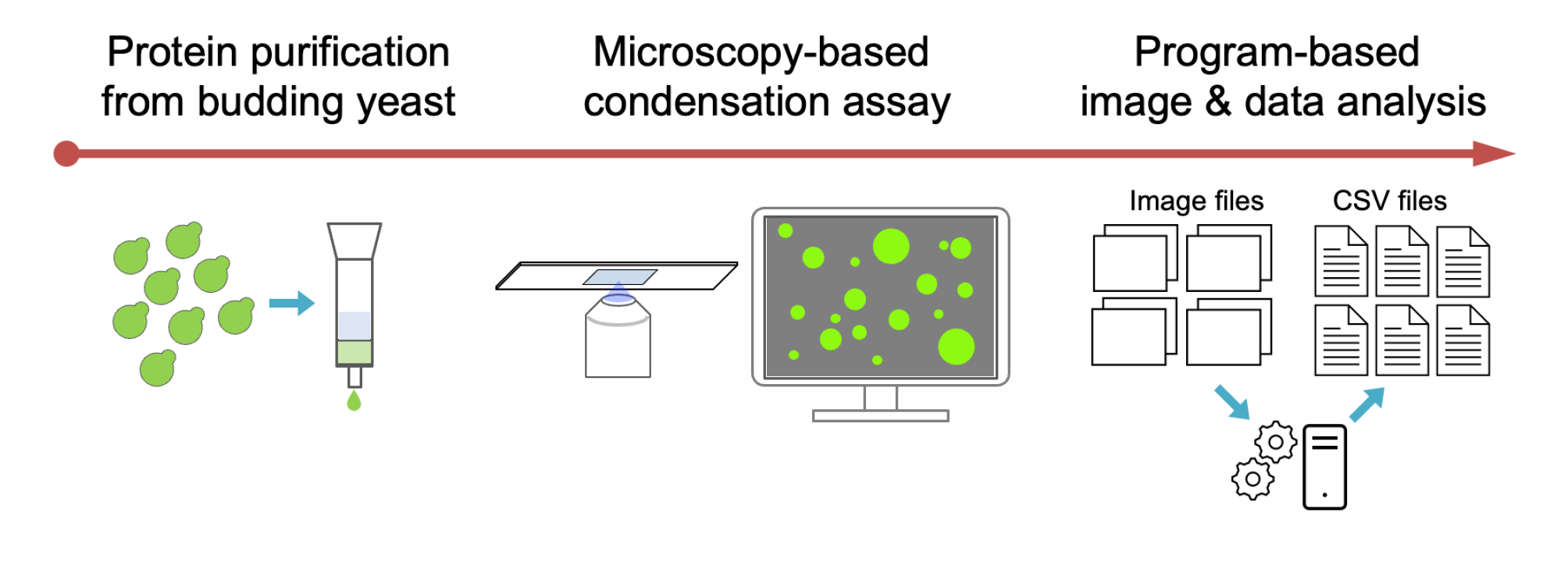
Workflow for purification of the fluorescent protein fused enzyme and in vitro condensation assay
Background
Purine nucleotides and their derivatives play crucial roles in various cellular functions, making them indispensable metabolites for all living organisms. These nucleotides are synthesized through both the salvage pathway and the de novo synthesis pathway. Under typical cellular conditions, the salvage pathway predominates, utilizing phosphoribosyl pyrophosphate (PRPP) to convert purine bases—often taken up from the extracellular environment—into purine nucleotides. However, when purine availability is limited or demand is elevated, such as in rapidly dividing cells, the de novo pathway is activated to ensure an adequate nucleotide supply [1]. Despite extensive research on the enzymes involved in purine biosynthesis, the precise regulatory mechanisms governing de novo purine synthesis remain incompletely understood.
PRPP amidotransferase (PPAT) (EC 2.4.2.14) catalyzes the initial and rate-limiting step of de novo purine biosynthesis, exerting a key regulatory function in this pathway. The enzyme’s biochemical properties and catalytic mechanisms have been extensively studied for decades, particularly through research using bacterial enzymes [2,3]. A notable characteristic of PPAT is its feedback inhibition by the end products of the de novo pathway, such as AMP [2–4]. This regulatory mechanism is thought to modulate de novo purine biosynthesis in response to extracellular purine availability, as observed in mammalian cell cultures [4]. However, the purification of eukaryotic PPAT has not yet been established, and its biochemical and biophysical properties remain largely uncharacterized.
A growing body of evidence suggests that many metabolic enzymes form condensates within cells in response to external stimuli to regulate cellular metabolism [5]. PPAT also reversibly localizes to cytoplasmic condensates upon depletion of extracellular purine bases in budding yeast and HeLa cells [6, 7]. However, attempts to express and purify yeast PPAT in bacteria have been unsuccessful [8], leaving the mechanism regulating yeast PPAT condensate formation and its physiological significance largely unknown.
Recently, we demonstrated that budding yeast PPAT, Ade4, self-assembles into micron-sized condensates through phase separation under molecular crowding conditions, leading to enzyme activation [9]. Purine nucleotides inhibit condensate formation, whereas PRPP promotes condensation, counteracting the inhibitory effects of purine nucleotides. To investigate this phenomenon, I developed a protocol to purify Ade4 tagged with the green fluorescent protein monomeric NeonGreen (mNG) from budding yeast cells using the Strep-tag®/Strep-Tactin® system [10], as well as a microscopy-based in vitro assay to examine the condensation of the fluorescent Ade4 protein. To our knowledge, this represents the first successful purification of a eukaryotic PPAT. This protocol can thus be adapted for the purification and condensation assays of PPAT from other species. Additionally, it offers a promising alternative for enzyme purification when bacterial expression proves unsuccessful, as was the case for yeast PPAT. This protocol is also useful when bacterial expression is inappropriate, for example, to investigate post-translational modifications of proteins specific to eukaryotic cells.
Several methods are available to study protein condensation in vitro, including bulk assays such as turbidity measurements and centrifugation, as well as fluorescence microscopy–based assays. Fluorescence microscopy–based assays, including the one introduced here, are especially useful as they allow direct observation of individual condensates, providing insights into condensate size, number, shape, and dynamic behavior. They can also reveal liquid-like properties and enable co-localization analysis by labeling different proteins with distinct fluorescent colors. Despite their strengths, fluorescence microscopy–based assays have limitations: they are low-throughput, less quantitative without image analysis, may miss small condensates, and often require labeling. Still, they remain key tools for understanding the mechanisms of protein condensation.
Materials and reagents
Biological materials
1. MTY3944 (MATa natNT2-PGPD-Ade4-mNG-Strep-tag II-hphNT1 his3∆1 leu2∆0 ura3∆0) (YGRC, BY29686)
2. MTY3969 (MATα his3Δ1::pRS303-PGPD-mNG-Strep-tag II-hphNT1 leu2Δ0 lys2Δ0 ura3Δ0) (YGRC, BY29688)
Note: MTY3944 and MTY3969 constitutively overexpress Ade4-mNG-Strep-tag II and mNG-Strep-tag II under the GPD promoter, respectively. Both yeast strains are available from the Yeast Genetic Resource Centre Japan (YGRC, http://yeast.nig.ac.jp/yeast/).
Reagents
1. Yeast extract (BD, catalog number: 212750)
2. Bacto-peptone (BD, catalog number: 211677)
3. D(+)-glucose (FUJIFILM Wako, catalog number: 049-31165)
4. Agar (FUJIFILM Wako, catalog number: 010-08725)
5. Adenine sulfate (FUJIFILM Wako, catalog number: 018-19613)
6. NaCl (FUJIFILM Wako, catalog number: 191-01665)
7. MgCl2·6H2O (FUJIFILM Wako, catalog number: 132-00175)
8. 0.5 M EDTA (DOJINDO, catalog number: 347-07481)
9. Ethanol, 99.5% (FUJIFILM Wako, catalog number: 057-00451)
10. 1 M Tris-HCl (pH 7.5) (NIPPON GENE, catalog number: 316-90221)
11. (+/-)-Dithiothreitol (FUJIFILM Wako, catalog number: 047-08973)
12. Benzylsulfonyl fluoride (aka phenylmethylsulfonyl fluoride, PMSF) (FUJIFILM Wako, catalog number: 028-15373)
13. PEG 8000 (FUJIFILM Wako, catalog number: 596-09755)
14. Buffer E (10×) (IBA GmbH, catalog number: 2-1000-025)
15. cOmplete protease inhibitor cocktail mini (EDTA-free) (Roche, catalog number: 11836170001)
16. Neutralized avidin (FUJIFILM Wako, catalog number: 015-24231)
17. Strep-Tactin Sepharose, 50% suspension (IBA GmbH, catalog number: 2-1201-002)
18. FastGene Q-stain (Nippon Genetics, catalog number: NE-FG-QS1)
19. Amicon Ultra-0.5 centrifugal filter device with a molecular weight cutoff of 30 kDa or 10 kDa [Merck, catalog number: UFC503024 (30 kDa) and UFC501008 (10kDa)]
20. Buffer R (10×) (IBA GmbH, catalog number: 2-1002-100)
21. Bovine serum albumin (BSA) standard solution (2 mg/mL) included in the Bradford Protein Assay Kit (TaKaRa, catalog number: T9310A)
Solutions
1. Adenine stock (see Recipes)
2. YPD agar plate (see Recipes)
3. YPDA (see Recipes)
4. 10× EB (see Recipes)
5. 0.5 M DTT (see Recipes)
6. EBD (see Recipes)
7. 0.1 M PMSF (see Recipes)
8. EBDPI (see Recipes)
9. EBDPIP (see Recipes)
10. 1 M MgCl2 (see Recipes)
11. EBMD (see Recipes)
12. EBM10D (see Recipes)
13. 50% PEG8000 (see Recipes)
14. 20% PEG8000 (see Recipes)
15. Buffer E (see Recipes)
16. Buffer R (see Recipes)
Recipes
1. Adenine stock (5 mg/mL)
Autoclave at 120 °C for 20 min.
| Reagent | Final concentration | Quantity or Volume |
|---|---|---|
| Adenine sulfate | 27.1 mM (in adenine base) | 0.5 g |
| H2O (deionized) | n/a | 99.75 mL |
2. YPD agar plate
Autoclave at 120 °C for 20 min. Pour the medium into a cell culture dish (approximately 20 mL/dish). Solidify the plates for 2–3 days before use, wrap in plastic wrap, and store at room temperature.
| Reagent | Final concentration | Quantity or Volume |
|---|---|---|
| Yeast extract | 1% (w/v) | 10 g |
| Bacto-peptone | 2% (w/v) | 20 g |
| D(+)-glucose | 2% (w/v) | 20 g |
| Agar | 2% (w/v) | 20 g |
| H2O (deionized) | n/a | 1 L |
3. YPDA
Add the adenine after autoclaving at 120 °C for 20 min.
| Reagent | Final concentration | Quantity or Volume |
|---|---|---|
| Yeast extract | 1% (w/v) | 10 g |
| Bacto-peptone | 2% (w/v) | 20 g |
| D(+)-glucose | 2% (w/v) | 20 g |
| H2O (deionized) | n/a | 1 L |
| 5 mg/mL adenine stock | 0.02 mg/mL | 4.02 mL |
4. 10× EB (20 mL)
Store at room temperature.
| Reagent | Final concentration | Quantity or Volume |
|---|---|---|
| NaCl | 1.5 M | 1.75 g |
| 0.5 M EDTA | 10 mM | 0.4 mL |
| 1 M Tris-HCl pH 7.5 | 400 mM | 8 mL |
| H2O (deionized) | n/a | Up to 20 mL |
5. 0.5 M DTT (20 mL)
Aliquot and store at -20 °C. Avoid repeated freeze-thaw cycles.
| Reagent | Final concentration | Quantity or Volume |
|---|---|---|
| (+/-)-Dithiothreitol | 1 M | 1.54 g |
| H2O (deionized) | n/a | 20 mL |
6. EBD (50 mL)
Store at 4 °C.
| Reagent | Final concentration | Quantity or Volume |
|---|---|---|
| 10×EB | 1× | 5 mL |
| 1 M DTT | 1 mM | 50 μL |
| H2O (deionized) | n/a | 44.95 mL |
7. 0.1 M PMSF (10 mL)
Caution: Be careful not to inhale the powder or allow it to come into contact with skin or eyes. Store at -20 °C.
| Reagent | Final concentration | Quantity or Volume |
|---|---|---|
| PMSF | 0.1 M | 0.174 g |
| Ethanol | n/a | 10 mL |
8. EBDPI (10 mL)
Dissolve the tablet in a 15 mL tube by gently stirring. Store at -20 °C.
| Reagent | Final concentration | Quantity or Volume |
|---|---|---|
| EBD | n/a | 10 mL |
| cOmplete protease inhibitor cocktail mini (EDTA-free) | n/a | 1 tablet |
9. EBDPIP (5 mL)
Use within 30 min after preparation.
| Reagent | Final concentration | Quantity or Volume |
|---|---|---|
| EBDPIP | n/a | 5 mL |
| 0.1 M PMSF | 1 mM | 50 μL |
10. 1 M MgCl2 (10 mL)
Store at room temperature.
| Reagent | Final concentration | Quantity or Volume |
|---|---|---|
| MgCl2·6H2O | 1 M | 2.03 g |
| H2O (deionized) | n/a | Up to 10 mL |
11. EBMD (10 mL)
Store at 4 °C.
| Reagent | Final concentration | Quantity or Volume |
|---|---|---|
| 10×EB | 1× | 1 mL |
| 1 M MgCl2 | 5 mM | 50 μL |
| 0.5 M DTT | 10 mM | 20 μL |
| H2O (deionized) | n/a | Up to 10 mL |
12. EBM10D (2 mL)
Store at 4 °C.
| Reagent | Final concentration | Quantity or Volume |
|---|---|---|
| 10×EB | 1× | 200 μL |
| 1 M MgCl2 | 5 mM | 10 μL |
| 0.5 M DTT | 10 mM | 40 μL |
| H2O (deionized) | n/a | 1.75 mL |
13. 50% PEG8000 (10 mL)
Mix all components except DTT in a 50 mL tube and incubate in a water bath for 20 min at 45 °C. Invert the tube repeatedly to dissolve the PEG. Allow to cool to room temperature and add DTT.
| Reagent | Final concentration | Quantity or Volume |
|---|---|---|
| PEG8000 | 50% (w/v) | 5 g |
| 10× EB | 1× | 1 mL |
| 1 M MgCl2 | 5 mM | 50 μL |
| 0.5 M DTT | 1 mM | 20 μL |
| H2O (deionized) | n/a | Up to 10 mL |
14. 20% PEG8000 (1 mL)
Pipette the viscous 50% PEG8000 using a 1,000 μL tip with the end cut off and mix with EBMD by repeated pipetting.
| Reagent | Final concentration | Quantity or Volume |
|---|---|---|
| 50% PEG8000 | 20% (w/v) | 0.4 mL |
| EBMD | n/a | 0.6 mL |
15. Buffer E (10 mL)
Store at 4 °C. Final composition: 2.5 mM D-desthiobiotin, 0.15 M NaCl, 1 mM EDTA, 100 mM Tris-HCl, 1 mM DTT, pH 8.0.
| Reagent | Final concentration | Quantity or Volume |
|---|---|---|
| Buffer E (10×) | 1× | 1 mL |
| 0.5 M DTT | 1 mM | 20 μL |
| H2O (deionized) | n/a | Up to 10 mL |
16. Buffer R (10 mL)
Store at 4 °C. Final composition: 1 mM hydroxy-azophenyl-benzoic acid (HABA), 0.15 M NaCl, 1 mM EDTA, 100 mM Tris-HCl, pH 8.0.
| Reagent | Final concentration | Quantity or Volume |
|---|---|---|
| Buffer R (10×) | 1× | 1 mL |
| H2O (deionized) | n/a | Up to 10 mL |
Laboratory supplies
1. Cell culture dish, sterilized (SANSEI MEDICAL CO., LTD., catalog number: 01-013)
2. Pipette tips [Watson® Bio Lab, catalog numbers: 123R-755YS (200 μL), 123R-757CS (1000 μL)]
3. Sterile culture tube (16 mL, polypropylene) (EVERGREEN, catalog number: 222-2393-080)
4. Erlenmeyer flask with baffle, 500 mL (SHIBATA, catalog number: 016310-500A)
5. Centrifuge tube, 50 mL, flat top, polypropylene (TRUELINE, catalog number: TR2005)
6. 2 mL tube with screw cap and O-ring, polypropylene (YASUI KIKAI, catalog number: STC-0250)
7. Glass beads (0.5 mm diameter) (YASUI KIKAI, catalog number: YGBLA05)
8. Cell counting slides for TC10™/TC20™ cell counter, dual chamber (Bio-Rad, catalog number: 1450015)
9. Slide glass (MATSUNAMI, catalog number: SFF-001)
10. Coverslip (No. 1 thickness) (MATSUNAMI, catalog number: C018181)
11. Double-sided tape, 5 mm wide (NICHIBAN, catalog number: NW-5)
12. Pasteur pipette, 150 mm (AS ONE, catalog number: 2-2045-01)
13. Silicon dropper, 1 mL (AS ONE, catalog number: 1-6227-02)
14. Empty gravity flow column (1.1 cm diameter and 4.5 cm height) (Amersham Pharmacia, catalog number: 27-4570-01 or equivalent)
15. Low protein binding tube, 1.5 mL (BMS, catalog number: Dot-LP150)
16. Low protein binding tube, 0.5 mL (BMS, catalog number: Dot-LP050)
17. Low protein binding pipette tip [BMS, catalog number: BC-UP-0110S (10 μL), BC-UP-2010S (200 μL), BC-UP-1010S (1000 μL)]
18. Toothpicks (6.5–18 cm) (any brand)
Note: Sterilize before use.
Equipment
1. Automated cell counter (Bio-Rad, model: TC-20)
2. Hybrid high-speed refrigerated centrifuge (KUBOTA, model: 6200)
3. Tabletop micro refrigerated centrifuge (KUBOTA, model: 3520)
4. Bench-top shaking water bath (TAITEC, model: Personal-11 SDN set)
5. VORTEX-GENIE 2 Mixer (M&S Instruments Inc., model: SI-0286)
6. Multi-beads shocker (YASUI KIKAI, model: MB901)
7. Inverted fluorescent microscope (Nikon, model: Eclipse Ti2-E) equipped with:
a. 100× objective lens (Nikon, model: CFI Plan Apoλ 100× Oil Ph3 DM/NA1.45)
b. High-pressure mercury lamp (Nikon, model: Intensilight C-HGFIE 130 W)
c. CMOS image sensor (Nikon, model: DS-Qi2)
d. FITC filter set (Nikon, model: Ex465-495/DM505/BA515-555)
8. Bench-top aspirator (INTEGRA, model: VACUSIP)
9. Inverted routine microscope (Nikon, Eclipse Ts2) equipped with a 40× objective lens (Nikon, CFI Achromat LWD ADL 40XF/NA 0.55, catalog number: MRP46402)
10. Autoclave (TOMY SEIKO CO., LTD, model: LBS-325)
11. Incubator (TAITEC, model: INCUBATE BOX M-200F)
12. Culture rotator (TAITEC, model: RT-50)
13. Rotary shaker (NISSIN, model: NX-20)
14. Blue LED illuminator (NIHON EIDO, model: NF-1050-B)
15. Dark box for LED illumination (NIHON EIDO, model: NF-1060)
16. Pipettes [BM EQUIPMENT Co., LTD, PipetPAL®, PAL-200 (20–200 μL), PAL-1000 (100–1,000 μL)]
17. Stand with flat table and steel support (AS ONE, catalog number: 6-425-03 or any brand)
18. One-sided opening clamp (AS ONE, catalog number: 6-776-05 or any brand)
19. Silicone tubing (any brand)
20. Paper clips (any brand)
Software and datasets
1. NIS-Element AR (Nikon, v. 4.30.01)
2. Fiji (Fiji contributors [11], v. 2.16.0/1.54g)
3. R programs (The R Foundation for Statistical Computing Platform, v. 4.3.3)
4. RStudio Desktop (Posit Software, v. 2023.09.0+463)
Procedure
A. Cell preparation
1. Streak budding yeast cells (MTY3944 or equivalent) from a frozen stock using a pipette tip on a YPD agar plate and incubate at 30 °C for 1–2 days until colonies form.
2. Preparation of the preculture: using a sterilized toothpick, transfer a small smear of cells from the plate into 2 mL of YPDA in a 16 mL culture tube. Incubate at 30 °C overnight (>16 h) with rotation at approximately 40 rpm using a rotator.
3. Dilute a small aliquot of the preculture 10-fold in YPDA (e.g., add 10 μL to 90 μL of YPDA). Measure the cell density using an automated cell counter.
4. Preparation of the main culture: dilute the preculture in 100 mL of YPDA to a final concentration of 5 × 10⁴ cells/mL in a 500 mL flask and incubate the culture at 30 °C for 15 h with shaking at approximately 180 rpm.
Note: Since the doubling time is approximately 1.5 h, the cell density after T h is 5 × 2T/1.5 × 104 cells/mL. Under optimal conditions, the cell density will reach 5 × 10⁷ cells/mL after 15 h.
5. Measure the cell density repeatedly as described in step A3 until it reaches 1 × 10⁸ cells/mL.
6. Collect cells by centrifugation of 25 mL of the culture twice at 2,000× g in a swing rotor, using two 50 mL tubes.
7. Suspend the cell pellet in a 50 mL tube with 1 mL of ice-cold EBD, then transfer the suspension into a 2 mL screw-cap tube.
8. Centrifuge the sample at 10,000× g for 1 min to pellet the cells. Discard the supernatant.
9. Suspend the cell pellet with 1 mL of EBDPI, then centrifuge again.
10. Discard the supernatant and proceed to cell extraction. A 100 mL culture yields two 2 mL tubes, each containing approximately 5 × 10⁹ cells. Pause point: The cell pellets can be stored at -80 °C.
Note: Whether the cells express green fluorescent proteins can be confirmed by illuminating the cell pellets with a blue LED and seeing whether they emit significant green fluorescence, as shown in Figure 1.
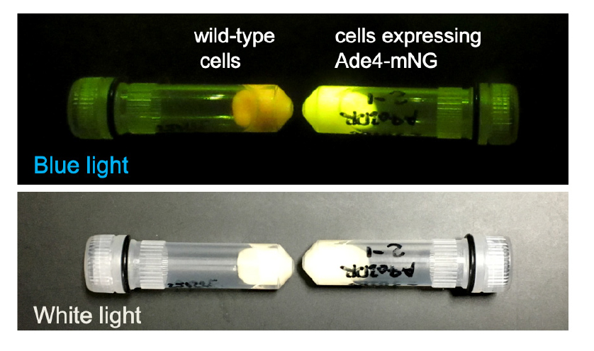
Figure 1. Cell pellets. Pellets of wild-type cells and cells expressing Ade4-mNG in a 2 mL tube were imaged under blue and white light illumination. Note that even the wild-type cell (BY4741) pellet shows weak green fluorescence derived from intrinsic fluorescence.
B. Cell extract preparation
1. Add 1.2 g of glass beads and 0.35 mL of EBDPIP to the cell pellet (approximately 5 × 10⁹ cells) in a 2 mL tube.
2. Disrupt cells by vigorous shaking using a bead beater. One beating session consists of 30 s of shaking at 2.7K rpm followed by a 30 s rest interval to prevent overheating and allow the sample to cool slightly. Repeat the beating session five times.
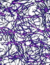
3. Remove the tube and take a small amount (<2 μL) of the cell suspension. Examine under a microscope to see if >70% of cells are disrupted (Figure 2).
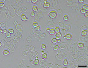
Figure 2. Yeast cell disruption. Intact cells appear shiny, while destroyed cells show only their empty shells. Scale bar = 10 µm.
4. If cell disruption is insufficient, repeat the beating session up to two additional times.
5. Transfer the crude cell homogenate into a 1.6 mL microtube using a 1,000 µL pipette tip.
6. Add 0.35 mL of EBDPIP to the remaining glass beads, mix thoroughly by vortexing, and transfer the liquid to the initial homogenate.
7. Centrifuge the sample at 20,000× g for 10 min at 4 °C.
8. Remove the supernatant (approximately 0.7 mL) and again centrifuge at 20,000× g for 10 min at 4 °C.
9. Remove the supernatant and add 1/49th volume of 10 mg/mL neutralized avidin, resulting in a final concentration of 0.2 mg/mL (2.9 µM).
Note: Endogenous biotin in cell extracts strongly, almost irreversibly, binds to Strep-Tactin resin and thereby prevents binding of the Strep-tag fusion protein and inactivating the resin. Therefore, the manufacturer strongly recommends masking the biotin by adding a stoichiometric amount of avidin. Wild-type budding yeast cells grown under normal conditions contain 0.62 ng of biotin per 1 × 10⁷ cells [12]. This concentration of avidin roughly corresponds to a 5-fold molar excess relative to the biotin in the supernatant, based on its four biotin-binding sites per molecule.
10. Incubate on ice for 30 min, inverting the tube occasionally.
11. Centrifuge at 20,000× g for 15 min at 4 °C and repeat this step once more.
12. Carefully remove only the clear supernatant. If starting with two 2 mL tubes, the final supernatant volume should be approximately 1.4 mL.
C. Construction of an open column for purification
1. Secure an empty gravity-flow column (commercial or handmade) in an upright position using a stand and clamp (Figure 3). Ensure that the bottom frit is in place to prevent resin leakage. Connect silicone tubing to the column outlet and keep it closed using a clip.
2. Close the column outlet and pipette 1 mL of a 50% suspension of Strep-Tactin Sepharose into the column.
3. Allow the resin to settle for 10 min to obtain a column bed volume (CV) of 0.5 mL.
4. Pipette 1 mL of EBD (2 CV) to wash the column before use.
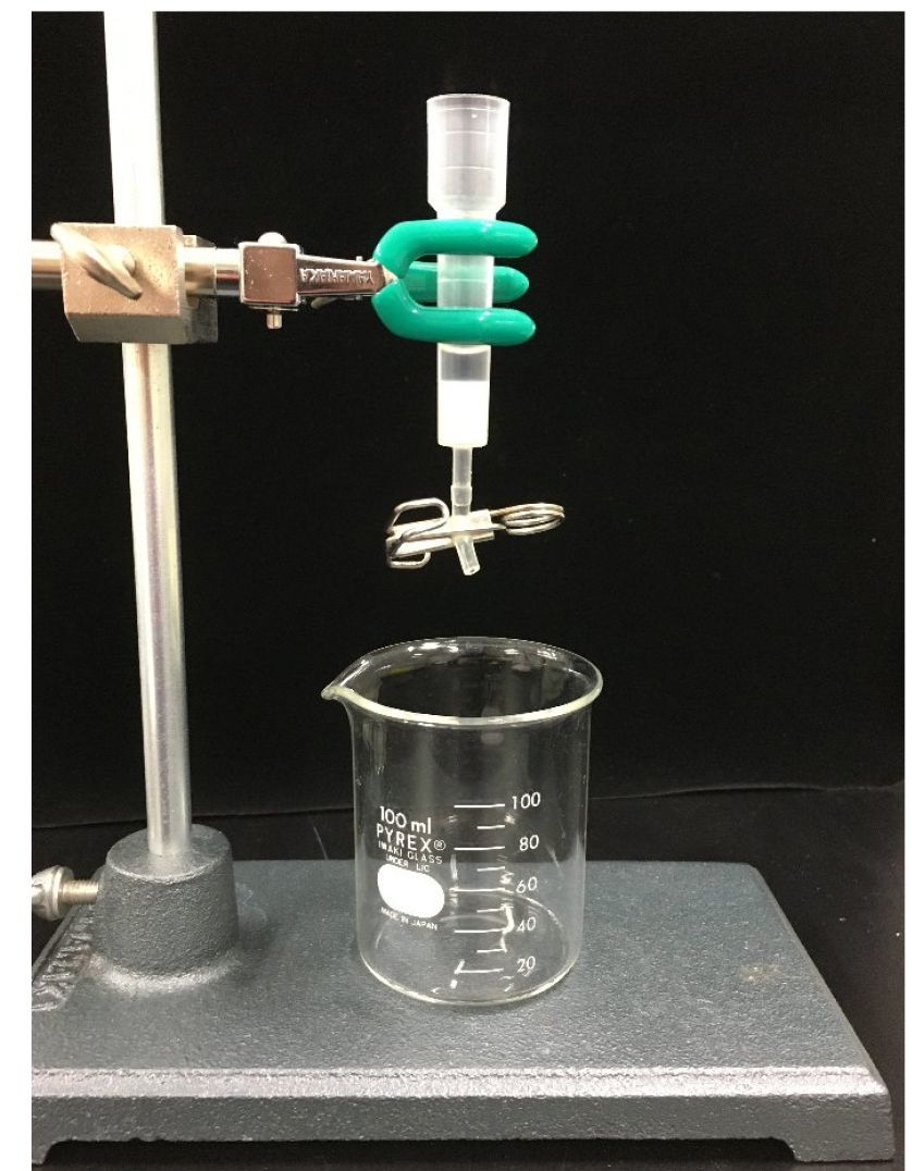
Figure 3. Overview of the open column system.
D. Purification of Ade4-mNG
1. Overlay 1.4 mL of the clarified cell extract onto the top of the column packed with 0.5 mL of Strep-Tactin Sepharose.
2. Allow the extract to flow through the column by gravity.
Note: Ade4-mNG in the extract will specifically bind to Strep-Tactin resin via the Strep-tag fused to its C-terminal.
3. Wash the column with 6 mL (12 CV) of EBD (Figure 4A): after all the extract has soaked into the column, using a Pasteur pipette, gently overlay 1 mL of EBD onto the top of the column. Wait for the EBD to permeate the column and repeat this step six times.
4. Elution with 3 mL (6 CV) of buffer E (Figure 4B): using a Pasteur pipette, gently load 0.5 mL of buffer E onto the top of the column. Collect the 0.5 mL eluate in a 1.5 mL low protein binding microtube. Repeat this step six times.
Note: D-desthiobiotin contained in the buffer E competitively displaces Ade4-mNG bound to the Strep-Tactin resin. Since Ade4-mNG is easily adsorbed, use low protein binding tubes or pipette tips for subsequent handling of the protein.
5. Add 2.5 μL of 1 M MgCl2 to each eluate.
Note: Millimolar concentrations of magnesium are required to maintain the enzymatic activity of PPAT [13].
6. For initial purification or pilot experiments, analyze the fractions by SDS-PAGE to determine peak fractions (Figure 4C).
Note: Alternatively, peak fractions can be determined by illuminating the eluates with a blue LED (Figure 4D, E).
7. Concentrate the peak fractions, usually the first and second fractions, using a centrifugal filter device with a 30 kDa molecular weight cutoff. Centrifuge twice with 0.5 mL portions at 14,000× g for 10 min at 4 °C.
Note: The protocol is also adaptable for the purification of mNG protein from MTY3969. The purified mNG protein serves as a negative control in some assays. As the molecular weight of the mNG-Strep tag is approximately 29.6 kD, it should be concentrated using a filter device with a molecular weight cutoff of 10 kDa.
8. When less than 50 μL concentrate remains, add 450 μL of EBM10D and concentrate again, repeating this process twice.
Note: This process reduces the concentration of D-desthiobiotin in the eluate by 100-fold and increases the concentration of DTT by 10-fold. The addition of reducing agents is important for PPAT stability [13].
9. Invert the filter device and centrifuge at 1,000× g for 2 min to recover the concentrate.
10. Centrifuge at 20,000× g for 15 min at 4 °C. The supernatant contains the purified Ade4-mNG fraction.
11. Determine the concentration of the purified protein by densitometry using bovine serum albumin (BSA) as a standard following SDS-PAGE and staining with the Q-stain (Figure 4F). The estimated molecular weight of Ade4-mNG is 86.2 kD, and a band should be detected at this molecular weight position.
Note: The author recommends using densitometry for protein quantification rather than bulk measurement methods such as Lowry, BCA, Bradford, or Nanodrop, because it is important to verify the protein purity in the purified fraction, and densitometry allows determination of the effective concentration of the protein of interest. FIJI has a set of commands useful for densitometry of one-dimensional gels (go to Analyze → Gels). The theoretical background and notes on densitometry are also explained in the online manual (https://imagej.net/ij/docs/guide/146-30.html#toc-Subsection-30.13).
12. Store the purified Ade4-mNG on ice and use it for in vitro assays within 2 days to minimize loss of activity. Pause point: The purified Ade4-mNG can be stored at -80 °C.
Note: Purified Ade4-mNG loses the condensation activity over time, so it must be stored frozen unless it is used in an assay within 2 days of purification (the day the purified protein is concentrated and the following day) (also, see the note in step E2a below).
13. Wash the column with 3.5 mL of buffer R containing the yellow azo dye hydroxyl-azophenylbenzoic acid (HABA) (Figure 4G). Close the column and store at 4 °C.
Note: When HABA binds to the resin and displaces desthiobiotin, the column turns red, indicating successful regeneration. The column can be regenerated 5–7 times. If reusing, wash the red column with at least 4 mL of EB until it returns to its white color.
Figure 5 shows a relationship between the total yield of Ade4-mNG purification and the number of cells contained in the initial cell pellets. The graph shows that in a typical purification, the initial 1010 cells yield approximately 25 μg of pure Ade4-mNG, which is enough for 90 runs of the assay described in the following section (see General note 3 for further discussion).
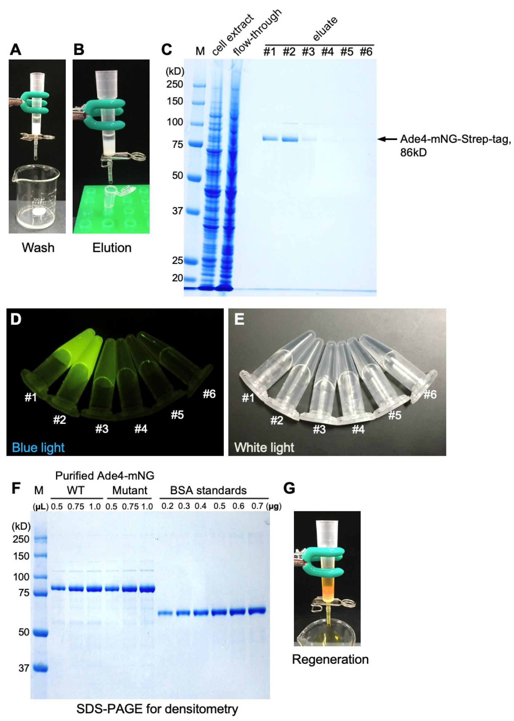
Figure 4. Purification of Ade4-mNG. (A) Washing of the column after loading of the cell extract. (B) Elution of the target protein. (C) SDS-PAGE analysis of cell extract, flowthrough, and the eluates. M, a protein molecular weight marker. (D, E) The eluates #1–6 in a microtube were imaged under blue and white light illumination. (F) SDS-PAGE of purified Ade4-mNG (wild type and the D373A/D374A mutant [9]) alongside BSA standards for densitometry-based quantification. Different volumes of purified proteins (0.5, 0.75, and 1.0 μL) and different known amounts of BSA (0.2–0.7µg) were loaded. (G) Regeneration of the column resin with buffer R.
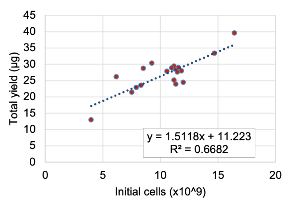
Figure 5. Total yield of Ade4-mNG purification. Scatter plot of the total yield of Ade4-mNG vs. the number of initial cells. Data from 19 independent purifications are plotted. The linear regression line, with the corresponding equation and R-squared value, is also plotted.
E. In vitro condensation assay
1. Preparation of assay chambers
a. Cut two pieces of 5 mm wide double-sided tape into 3–4 cm length sections.
b. Attach the tape pieces to a slide glass, positioning them 4 mm apart.
c. Place a coverslip (18 × 18 mm) onto the slide to form a chamber with an approximate volume of 9 μL (Figure 6).
d. Assemble the required number of chambers before starting the experiment.
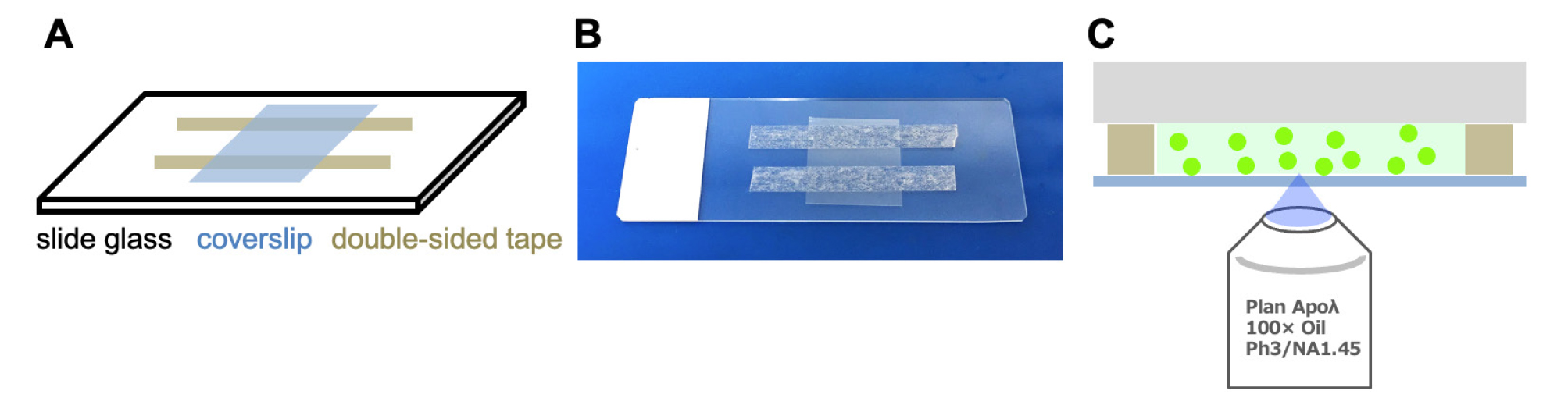
Figure 6. Handmade assay chamber. (A) Schematic of the chamber. (B) The actual chamber. (C) Observation of the coverslip surface inside the chamber.
2. Fluorescence microscopy of condensates
a. Dilute the purified Ade4-mNG to 3 μM (approximately 0.26 mg/mL) in EBM10D to create a 15× stock solution.
Note: 20–25 μL aliquots of the 15× stock of Ade4-mNG dispensed in a 0.6 mL tube can be frozen and stored by directly placing them into a -80 °C freezer. If using frozen stocks, thaw them quickly by immersing the 0.6 mL tube in 35 °C water and then placing on ice for 4–5 h prior to assay (see General note 1). Use it within 24 h of thawing.
b. Dilute the Ade4-mNG stock in the assay buffer (e.g., EBMD) in the presence of a reagent to be tested.
c. Mix with an equal volume of crowding agent (e.g., PEG8000) at two times the final concentration to initiate condensation. An example of a recipe is shown in Table 1.
Table 1. Example of mixture recipe for the assay. Mix from top to bottom.
| Reagent | Mock | +AMP | +CMP |
|---|---|---|---|
| EBMD | 5.5 μL | 5.5 μL | 5.5 μL |
| EBMD | 1 μL | - | - |
| 7.5 mM AMP (15× stock) | - | 1 μL | - |
| 7.5 mM CMP (15× stock) | - | - | 1 μL |
| 3 µM Ade4-mNG | 1 μL | 1 μL | 1 μL |
| 20% PEG8000 | 7.5 μL | 7.5 μL | 7.5 μL |
| Total | 15 μL | 15 μL | 15 μL |
d. Immediately load 9 μL of the sample into the chamber.
Note: Capillary action draws the sample into the chamber.
e. Invert the chamber and mount on an inverted fluorescent microscope.
f. Leave the chamber for 2 min. During this time, focus on the coverslip surface inside the chamber with a 100× objective lens with a numerical aperture of 1.45 (Figure 6C).
g. After the 2 min incubation, begin observing green fluorescence and focus on the fluorescent condensates.
h. Acquire both green fluorescence and phase contrast images of the condensates from a single z-plane.
Note: The combined images (green fluorescence and phase contrast) are automatically saved as an .nd2 file.
i. Move to an unimaged field of view, focus on the condensates, and acquire additional images.
j. For each experimental condition, collect images from multiple fields of view.
Data analysis
A. Image analysis
The first step in data analysis is image analysis. From the digital images of the condensates, we aim to extract information about the fluorescence intensity (the total amount of fluorescent protein in the condensate) and the shape of individual condensates. For this purpose, the images are analyzed using the open-source platform FIJI [11]. The following section explains how to manually analyze a single file for image analysis to make the process easier for the reader to understand. However, the actual analysis involves batch processing of multiple files by running a macro script.
1. Open an .nd2 file using FIJI as a hyperstack file (multi-channels) and split it into each channel image of 16-bit depth (one green fluorescence image and one phase contrast image) by going to Image → Color → Split Channels.
2. Save the phase contrast image as a TIFF file and close the window.
Note: The phase contrast image is not required for analysis of fluorescent condensates, but is useful for checking contamination and ensuring proper focus.
3. Save the green fluorescence image as a TIFF file.
4. Make a copy of the green fluorescence image by going to Image → Duplicate and enter a name in the Title box (e.g., “bin_image”) (Figure 7A). This duplicated image is used to create a binary image of condensates. Perform the following steps 5–11 on this image.
5. Subtract the background using the rolling-ball algorithm (Figure 7B): Process → Subtract Background. Set the rolling ball radius to 20 pixels and check the Disable smoothing box.
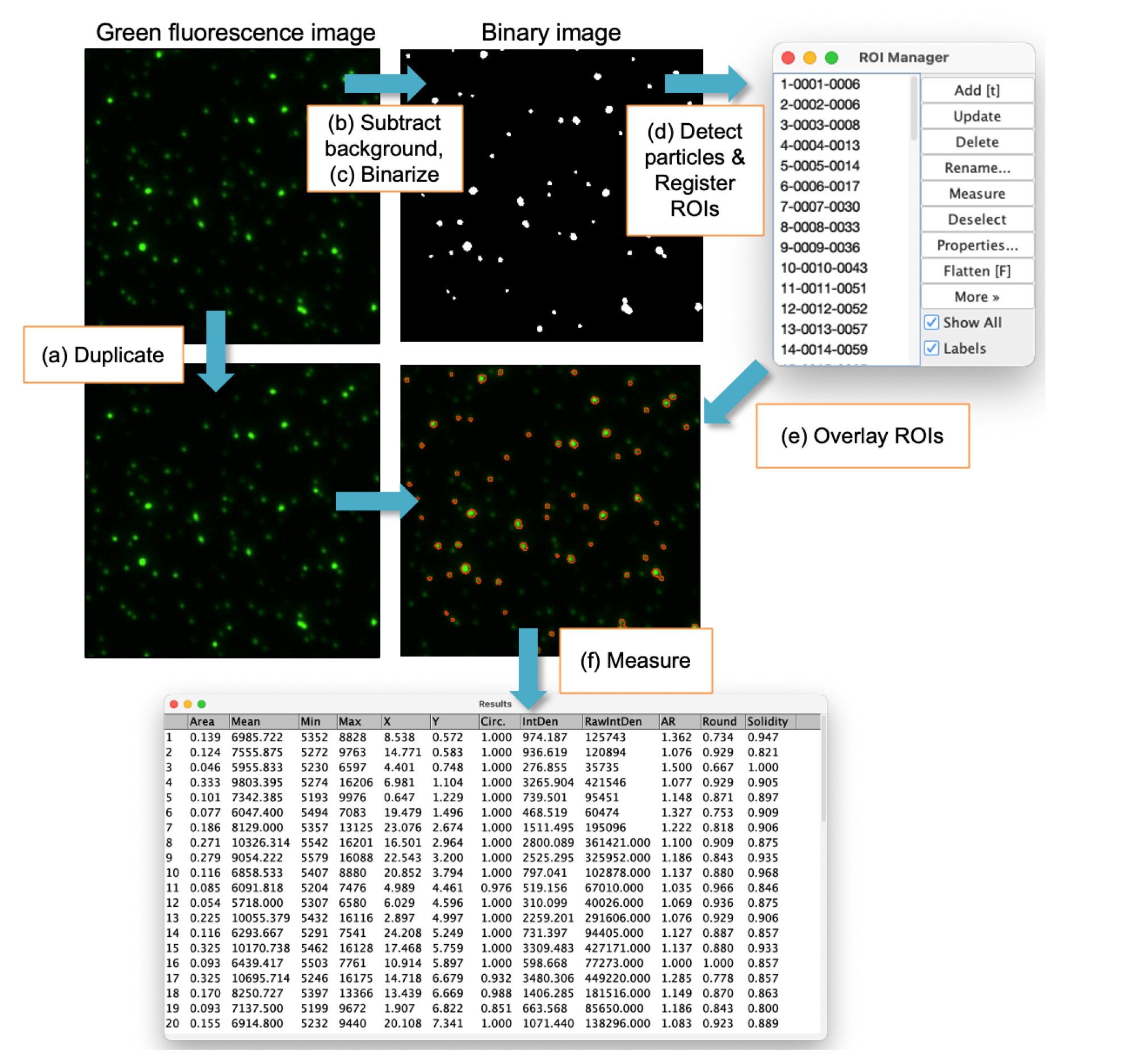
Figure 7. Workflow for image analysis in FIJI. Overview of the analysis steps performed after step 4. (A) Duplicate: Create a copy of the original image for binary conversion. (B) Subtract background: Apply the rolling-ball algorithm to remove local background and correct uneven illumination. (C) Binarize: Convert the image to binary by setting pixels within the defined threshold range to white and all others to black. (D) Detect particles and register ROIs: Identify white condensates in the binary image and add the corresponding ROIs to the ROI Manager. (E) Overlay ROIs: Overlay the ROIs onto the original fluorescence image to enable intensity measurements. (F) Measure: Measure morphological parameters and fluorescence intensities of all detected condensates simultaneously.
6. View the histogram by going to Analyze → Histogram.
7. Record the values of Mean and StdDev in the histogram. Calculate the threshold parameter LT using the equation: LT = Mean + 3×StdDev. See General note 4 for further clarification.
8. Convert the image into a binary image (Figure 7C): Go to Image → Adjust → Threshold. Check the Dark background and Raw values check boxes, then click Set. Set the Lower threshold level to LT and Upper threshold level to 65535. Click OK and then click Apply.
9. Set the measurements by going to Analyze → Set Measurements, check Area, Mean gray value, Min & max gray value, Centroid, Shape descriptor, Integrated density. Set Redirect to: to None and click OK.
Note: Measurement of all morphological parameters is encouraged for future exploratory data analysis and data mining.
10. Detect particles (condensates) in the binary image and examine their shape: Go to Analyze → Analyze particles (Figure 7D). Set Size to 0.04–500, uncheck Pixel units. Set Circularity to 0.1–1.00. Set Show: to Masks. Check Exclude on edges, Clear results, and Add to Manager. Uncheck Display Results. Click OK.
Note: The above settings target particles with a size of 0.04–500 µm2 and a circularity of 0.1–1.0 for detection. This process generates regions of interest (ROIs) of the detected condensates and registers these ROIs in the ROI manager. See General note 4 for additional clarification.
11. Save the binary image as a TIFF file and close the window.
12. Click on the original green fluorescence image window to bring it to the front.
13. Overlay all ROI stored in the ROI manager on the image (Figure 7E): In the ROI manager, click Deselect and then check Show All box.
14. Measure the shape of these ROIs and pixel values of the image inside the ROIs (Figure 7F): Click Measure in the ROI manager. The results will be displayed in the Results window.
15. Save the data as a text file in the comma-separated value (csv) format by clicking the Results window and then going to File → Save as.
Note: A macro script to automatically perform steps 1–15 repeatedly on multiple .nd2 files is available from the author’s GitHub site: https://github.com/masaktakaine/In-vitro-condensates-quantification.
B. Data presentation and statistical analysis
A single run of the image analysis described in the previous section yields a .csv file that summarizes the parameters that represent the intensity and shape of the condensate visualized in a single microscope field. The total number of .csv files obtained from an experiment increases depending on the number of experimental conditions, replicates (independent preparations of an assay), and number of microscopic fields imaged, sometimes amounting to hundreds. The author analyzes the multi-dimensional data using R programs and RStudio software [14]. To evaluate condensate assembly, the following two parameters that characterize condensates are typically reported:
1. The mean intensity of each condensate.
2. The sum of the integrated intensities of each condensate per image.
The mean intensity is the Mean grey value measured with FIJI (see the previous section) and represents the fluorescent protein concentration in the condensate. These values are sometimes reported after averaging over each image. The sum of the integrated intensities of each condensate per image is calculated using R programs and represents the total mass of the condensates detected in each image.
The following section describes an example of analyzing a total of 118 .csv files obtained by observing 34–44 fields of view each from three preparations under three experimental conditions [mock, adenosine monophosphate (AMP), or cytidine monophosphate (CMP) added]. The .csv files and the R script used for analysis are provided as Supplementary material Dataset S1. Below, important code chunks of the script are explained.
1. Make a project for data analysis in RStudio.
a. Create a new folder and put all the .csv files in it. Name the folder (e.g., image_data_csv).
b. Create another new folder, put the R script file and the .csv folder in it, and name the folder (e.g., 250428_data_ analysis).
c. In RStudio, link the folder to a new project by going to File → New Project → Existing directory → Browse, select the 250428_data_analysis, and click Create Project. This creates an .Rproj file in the folder with the same name as the folder (in this case, 250428_data_analysis.Rproj).
d. Shut down RStudio and double-click the Rproj file. Confirm that RStudio is running with the 250428_data_analysis as the working directory.
Note: The Rproj file allows you to set a specific folder as a working folder and restrict all file operations to that folder and its subfolders, making file management easier.
2. Open the R script file in the working directory by clicking Files in the Output panel at the lower right. Click the .R file. Alternatively, create a new R script by clicking File → New File → R script and copy the following code into the source window.
3. Load libraries required for analysis using the pacman::p_load function. To run the code, place the cursor on the line and press Command+Enter (⌘↵) for Mac or Ctrl+Enter for Windows.
Note: The readers are encouraged to run the codes in the script chunk by chunk in this way, although all codes in the script can be run at once by using Run All command by pressing Option+Command+R (⌥⌘R).
library(pacman)
p_load(tidyverse, openxlsx, ggsignif, ggpmisc, nparcomp, rstatix)
4. Import and combine the .csv files into a single dataframe object df_concat. This dataframe contains all the information (measurements) of each individual condensate in one row.
import_file_path <- "image_data_csv"
csv_list <-
list.files(import_file_path, full.names = T, pattern = "*.csv")
df_concat <-
csv_list %>%
sapply(., read.csv, header=T, sep = ",", stringsAsFactors = F, simplify = F) %>%
bind_rows()
5. Create a new parameter (column) “reagent” that represents three experimental conditions in the df_concat.
Note: The parameter “file” indicates the name of the image file analyzed. This code parses the file to see if it contains a particular word (e.g., “amp”), and if found, provides the corresponding value (e.g., “+AMP”) in the parameter reagent.
df_concat <-
df_concat %>%
mutate(reagent =case_when(
str_detect(file, "amp") ~ "+AMP",
str_detect(file, "cmp") ~ "+CMP",
TRUE ~ "Mock")
)
6. Calculate the average of the mean intensity of each condensate per image (Mean_mean), the sum of the integrated intensities of each condensate per image (IntDen_sum), and the number of condensates detected in the image (N_condensate). Store these data in a dataframe data_sum_per_image.
Note: The dataframe object (or any other dataframe) can be saved as an Excel file if desired.
# Calculation of Mean_mean, IntDen_sum and N_condensate
data_sum_per_image <-
df_concat %>%
dplyr::select(Area, Mean, IntDen, reagent, file) %>%
group_by(reagent, file) %>%
summarise_all(list(mean=mean, sum=sum, N_condensate = ~n())) %>%
rename(N_condensate = Area_N_condensate) %>%
dplyr::select(reagent:N_condensate, -Area_sum, -Mean_sum)
# Export of the dataframe as an Excel file.
data_sum_per_image %>%
write.xlsx("data_sum_per_image.xlsx", colNames = T)
7. Further calculate the mean and standard deviation (SD) of the parameters across 34–44 images under each condition based on the data in the data_sum_per_image.
# Calculation of the mean and SD.
mean_sd_per_image <-
data_sum_per_image %>%
dplyr::select(-file) %>%
group_by(reagent) %>%
summarise_all(list(mean=mean, sd=sd, N_field = ~n())) %>%
rename(N_field = Area_mean_N_field) %>%
dplyr::select(reagent:N_field)
mean_sd_per_image %>%
write.xlsx("mean_sd_per_image.xlsx", colNames = T)
8. Examine whether the data (Mean_mean and IntDen_sum) follow a normal distribution using the Shapiro–Wilk normality test. Results indicated that both variables were normally distributed in the mock and +AMP groups, whereas normality could not be confirmed in the +CMP group. These findings prompted the use of non-parametric methods for subsequent analyses.
# Normality test using the Shapiro-Wilk Normality test.
#Create a function to test the distribution of Mean_mean using rstatix::shapiro.test().
stest_mm <-
function(cond){data_sum_per_image %>%
filter(reagent == cond) %>%
ungroup() %>%
dplyr::select(Mean_mean) %>%
as_vector() %>%
shapiro.test()}
stest_mm("Mock") # p = 0.5786
stest_mm("+AMP") # p =0.1765
stest_mm("+CMP") # p =0.03352
# Create a function to test the distribution of IntDen_sum using the shapiro.test().
stest_is <-
function(cond){data_sum_per_image %>%
filter(reagent == cond) %>%
ungroup() %>%
dplyr::select(IntDen_sum) %>%
as_vector() %>%
shapiro.test()}
stest_is("Mock") # p = 0.456
stest_is("+AMP") # p= 0.07075
stest_is("+CMP") # p= 0.02768
9. Examine whether there is a statistically significant difference among the three conditions using the Kruskal–Wallis test, a non-parametric alternative to one-way analysis of variance (ANOVA). In this example, significant differences were observed for both parameters.
# Kruskal-Wallis test of Mean_mean
res_kw_mm <-
data_sum_per_image %>%
kruskal.test(data = ., Mean_mean ~ reagent)
res_kw_mm
# Output
Kruskal-Wallis rank sum test
data: Mean_mean by reagent
Kruskal-Wallis chi-squared = 74.32, df = 2, p-value < 2.2e-16
# Kruskal-Wallis test of IntDen_sum
res_kw_intden <-
data_sum_per_image %>%
kruskal.test(data = ., IntDen_sum ~ reagent)
res_kw_intden
# Output
Kruskal-Wallis rank sum test
data: IntDen_sum by reagent
Kruskal-Wallis chi-squared = 73.057, df = 2, p-value < 2.2e-16
10. Calculate p-values of the two reagent groups vs. mock using the Steel test, a non-parametric alternative to Dunnett’s test, which is a post-hoc test commonly used to compare multiple treatment groups against a single control group following a significant overall difference.
# Steel test of Mean_mean
res_st_mm <-
data_sum_per_image %>%
nparcomp(Mean_mean ~ reagent, data = ., asy.method = "mult.t",
type = "Dunnett",control = "Mock", alternative = "two.sided", info = FALSE)
summary(res_st_mm)
# A part of Output
# Comparison Estimator Lower Upper Statistic p.Value
# 1 p( Mock , +AMP ) 0.001 0.000 0.002 -1714.12129 1.110223e-16
# 2 p( Mock , +CMP ) 0.357 0.218 0.496 -2.35118 4.239875e-02
# Steel test of IntDen_sum
res_st_intden_sum <-
data_sum_per_image %>%
nparcomp(IntDen_sum ~ reagent, data = ., asy.method = "mult.t",
type = "Dunnett",control = "Mock", alternative = "two.sided", info = FALSE)
summary(res_st_intden_sum)
# A part of Output
# Comparison Estimator Lower Upper Statistic p.Value
# 1 p( Mock , +AMP ) 0.001 0.000 0.002 -1714.121291 0.0000000
# 2 p( Mock , +CMP ) 0.409 0.265 0.552 -1.454541 0.2764984
11. Plot the Mean_mean with p-values annotated (Figure 8A). Bars and error bars indicate the mean ± 1SD. If the graph is not shown, click Plots in the Output panel.
Note: The following code generates a bar graph showing the mean values with error bars, overlaid with individual data points displayed as a dot plot. This type of graph simultaneously presents the mean and variability while visualizing the distribution of individual data points. It allows intuitive understanding of data spread, sample size, and outliers, ensuring accurate group comparisons. For these reasons, it was extensively used in the original paper [9].
annot1 = c("<1.0e-10", "0.04")
y_position1 = c(8300, 7800)
xmin1 = c(1, 1)
xmax1 = c(2, 3)
plot_mean <-
mean_sd_per_image %>%
ggplot(aes(x= reagent, y=Mean_mean_mean, fill = reagent))+
geom_bar(aes(fill=reagent),stat="identity",color="black",width= 0.8,
position = position_dodge(width = 0.9))+
geom_signif(xmin = xmin1, xmax =xmax1, y_position =y_position1,
annotations = annot1, tip_length = 0.01, textsize = 4)+
geom_errorbar(limits_mean_mean,width=0.3,position=position_dodge(width=0.9))+
geom_jitter(data_sum_per_image,mapping=aes(x=reagent,y=Mean_mean, fill=reagent),size = 1.5, alpha=0.7, width = 0.2, height = 0)+
scale_fill_manual(values = c("#bdbdbd","#5da6f4", "#F8766D"))+
ylab("Mean density of \ncondensates/image") +
xlab("")+theme(axis.title.y=element_text(size=14),axis.text.y=element_text(size=14,
color="black"),axis.title.x=element_text(size=14),axis.text.x=element_text(size=14,
color = "black"),legend.position = "none", panel.border = element_rect(fill = NA, size = 0.5),panel.background = element_blank())
plot_mean
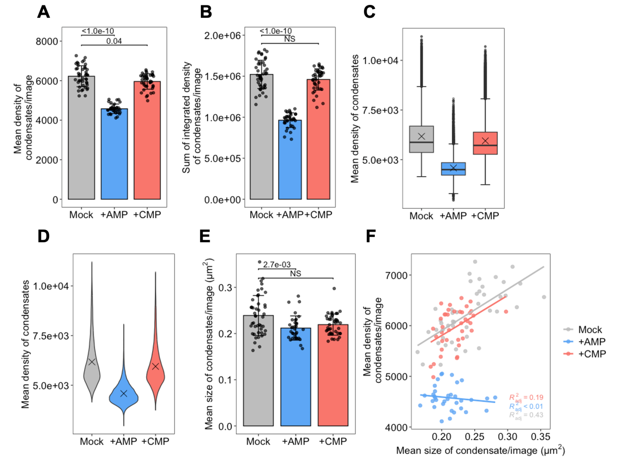
Figure 8. Various types of plots. (A) Mean intensities of condensates averaged per image. (B) Integrated intensities of condensates summed per image. (C) Boxplots of the mean intensities of condensates. (D) Violin plots of the mean intensities of condensates. Cross marks in C and D indicate the population mean. (E) Mean size of condensates averaged per image. (F) Scatter plot showing the mean intensity of condensates (averaged per image) plotted against the mean size of condensates (averaged per image), with linear regression lines superimposed. The coefficients of determination (R2) are indicated in the lower-right corner. Bars and error bars in panels A, B, and E indicate the mean ± 1SD. P-values in panels A, B, and E were calculated using the two-tailed Steel’s multiple comparison test.
12. Plot the IntDen_sum with p-values annotated (Figure 8B). Bars and error bars indicate the mean ± 1SD.
annot2 = c("<1.0e-10", "NS")
y_position2 = c(2.0e+06, 1.9e+06)
xmin2 = c(1, 1)
xmax2 = c(2, 3)
plot_intden_sum <-
mean_sd_per_image %>%
ggplot(aes(x= reagent, y=IntDen_sum_mean, fill=reagent))+
geom_bar(stat="identity",color="black",width=0.8,
position = position_dodge(width = 0.9))+
geom_jitter(data_sum_per_image, mapping=aes(x=reagent, y= IntDen_sum),size = 1.5, alpha=0.7, width = 0.2, height = 0)+
geom_signif(xmin = xmin2, xmax =xmax2, y_position =y_position2,
annotations = annot2, tip_length = 0.01, textsize = 4)+
geom_errorbar(limits_sum_intden,width=0.3,position=position_dodge(width=0.9))+
scale_fill_manual(values = c("#bdbdbd","#5da6f4", "#F8766D"))+
ylab("Sum of integrated density\n of condensates/image") +
xlab("")+
scale_y_continuous(labels = scales::scientific_format())+
theme(axis.title.y=element_text(size=14),axis.text.y=element_text(size=14,
color="black"),axis.title.x=element_text(size=14),axis.text.x=element_text(size=14,
color = "black"),legend.position = "none", panel.border = element_rect(fill = NA, size = 0.5),panel.background = element_blank())
plot_intden_sum
13. Save the graph as an image file by clicking Export → Save as Image in the Plots panel. Select Image format (PNG, JPEG, TIFF, etc.), Directory, File name, Width, and Height (in pixels) and then press Save.
The resulting Figure 8A, B shows a statistically significant decrease in both the mean intensity and the sum of the integrated intensities for each condensate per image in the presence of AMP. In contrast, in the presence of CMP, the mean intensity is only slightly reduced, and the integrated densities remain unchanged. These results suggest that purine nucleotide (AMP) inhibits the in vitro condensation of Ade4-mNG as described in the original paper [9], while pyrimidine nucleotide (CMP) has no effect on the condensation. With minor modifications to the code, other types of plots can be created, such as boxplots and violin plots, as shown in Figure 8C, D (note that the values of Mean are not averaged per image in these plots). Boxplots and violin plots share common strengths when analyzing datasets with many data points. Both offer visual summaries of data distributions, making it easier to compare multiple groups or conditions. Boxplots highlight key statistical measures such as the median, interquartile range, and potential outliers. In contrast, violin plots provide a more detailed view of the distribution’s shape, revealing whether the data is skewed, symmetric, or multimodal.
In addition to intensity-related parameters, morphological parameters—which are generally independent of intensity parameters—should also be analyzed. For example, plots of the mean size (area on a two-dimensional plane) of condensates (averaged per image) are shown in Figure 8E. These data suggest that AMP, but not CMP, causes a slight yet significant decrease in condensate size. Furthermore, by using a morphological parameter as the x-axis variable, the relationship between condensate morphology and intensity can be examined. As an example, the scatter plot with linear regression lines shown in Figure 8F illustrates the relationship between the mean size and mean intensity of condensates (both averaged per image). These data suggest that the intensity of condensates increases roughly in proportion to their size under mock conditions and in the presence of CMP, whereas this positive correlation is lost in the presence of AMP, likely contributing to the significant reduction in the integrated density of condensates observed with AMP.
Validation of protocol
This protocol has been used and validated in the following research article:
Takaine et al. [9]. Phase separation of the PRPP amidotransferase into dynamic condensates promotes de novo purine synthesis in yeast. PLOS Biol (Figures 3, 6, and 7 and Supplementary Figures S5 and S10–S13).
General notes and troubleshooting
General notes
1. Ade4-mNG prepared from frozen stock may be insensitive to the ligand (purine nucleotide; see the background section or the original paper [9]) if used immediately after thawing. The exact mechanism of this insensitivity remains unclear, but incubation on ice for several hours resolves this issue.
2. Constitutive overexpression under the strong GPD promoter increases purification yields and can be adapted for the expression of proteins other than Ade4-mNG. However, if the expression of the protein of interest is toxic to yeast cells, transient expression using an inducible promoter such as the GAL1 promoter [15] should be considered.
3. Although the protein yield achieved by the current protocol is sufficient for the microscopy-based condensation assay, it remains lower than that typically obtained with bacterial expression systems. If a higher yield is required, the reader can scale up the initial culture up to 20-fold—preparing an extract from a 2 L culture and loading it onto a column of the same size—as the 0.5 mL resin still has sufficient binding capacity to accommodate this increase. Alternatively, the reader can increase the yield by enhancing the intracellular copy number of the expression construct.
4. The intensity threshold used to separate condensates from background was determined according to the so-called three sigma rule of thumb. It is reasonable to consider pixels that are more than three standard deviations above the image mean intensity as belonging to condensates, as bright condensates are sparsely scattered on a dark background in a typical image. However, when analyzing fluorescent condensates of other proteins, adjustment of the intensity threshold may be necessary (e.g., Mean+2×StdDev or Mean+6×StdDev). This need for adjustment also applies to the minimum size of particles to be detected.
5. In vitro assays using handmade chambers are simple and cost-effective, but are limited by (1) the inability to change the buffer in the chamber and (2) low observation throughput.
Supplementary information
The following supporting information can be downloaded here:
1. Dataset S1: csv files and R script file used in subsection B, “Data presentation and statistical analysis,” of the Data analysis section.
Acknowledgments
This work was supported by research grants from the Gout and Uric Acid Foundation of Japan and by JSPS KAKENHI Grant Number JP22K06216 to M.T. This work was also supported by the joint research program of the Institute for Molecular and Cellular Regulation, Gunma University, Japan.
Competing interests
The author declares no conflicts of interest.
References
- Pedley, A. M. and Benkovic, S. J. (2017). A New View into the Regulation of Purine Metabolism: The Purinosome. Trends Biochem Sci. 42(2): 141–154. https://doi.org/10.1016/j.tibs.2016.09.009
- Meyer, E. and Switzer, R. L. (1979). Regulation of Bacillus subtilis glutamine phosphoribosylpyrophosphate amidotransferase activity by end products.. J Biol Chem. 254(12): 5397–5402. https://doi.org/10.1016/s0021-9258(18)50609-8
- Messenger, L. J. and Zalkin, H. (1979). Glutamine phosphoribosylpyrophosphate amidotransferase from Escherichia coli. Purification and properties.. J Biol Chem. 254(9): 3382–3392. https://doi.org/10.1016/s0021-9258(18)50771-7
- Yamaoka, T., Yano, M., Kondo, M., Sasaki, H., Hino, S., Katashima, R., Moritani, M. and Itakura, M. (2001). Feedback Inhibition of Amidophosphoribosyltransferase Regulates the Rate of Cell Growth via Purine Nucleotide, DNA, and Protein Syntheses. J Biol Chem. 276(24): 21285–21291. https://doi.org/10.1074/jbc.m011103200
- Prouteau, M. and Loewith, R. (2018). Regulation of Cellular Metabolism through Phase Separation of Enzymes. Biomolecules. 8(4): 160. https://doi.org/10.3390/biom8040160
- Narayanaswamy, R., Levy, M., Tsechansky, M., Stovall, G. M., O'Connell, J. D., Mirrielees, J., Ellington, A. D. and Marcotte, E. M. (2009). Widespread reorganization of metabolic enzymes into reversible assemblies upon nutrient starvation. Proc Natl Acad Sci USA. 106(25): 10147–10152. https://doi.org/10.1073/pnas.0812771106
- An, S., Kumar, R., Sheets, E. D. and Benkovic, S. J. (2008). Reversible Compartmentalization of de Novo Purine Biosynthetic Complexes in Living Cells. Science. 320(5872): 103–106. https://doi.org/10.1126/science.1152241
- Rébora, K., Desmoucelles, C., Borne, F., Pinson, B. and Daignan-Fornier, B. (2001). Yeast AMP Pathway Genes Respond to Adenine through Regulated Synthesis of a Metabolic Intermediate. Mol Cell Biol. 21(23): 7901–7912. https://doi.org/10.1128/mcb.21.23.7901-7912.2001
- Takaine, M., Morita, R., Yoshinari, Y. and Nishimura, T. (2025). Phase separation of the PRPP amidotransferase into dynamic condensates promotes de novo purine synthesis in yeast. PLoS Biol. 23(4): e3003111. https://doi.org/10.1371/journal.pbio.3003111
- Schmidt, T. G. and Skerra, A. (2007). The Strep-tag system for one-step purification and high-affinity detection or capturing of proteins. Nat Protoc. 2(6): 1528–1535. https://doi.org/10.1038/nprot.2007.209
- Schindelin, J., Arganda-Carreras, I., Frise, E., Kaynig, V., Longair, M., Pietzsch, T., Preibisch, S., Rueden, C., Saalfeld, S., Schmid, B., et al. (2012). Fiji: an open-source platform for biological-image analysis. Nat Methods. 9(7): 676–682. https://doi.org/10.1038/nmeth.2019
- Pirner, H. M. and Stolz, J. (2006). Biotin Sensing in Saccharomyces cerevisiae Is Mediated by a Conserved DNA Element and Requires the Activity of Biotin-Protein Ligase. J Biol Chem. 281(18): 12381–12389. https://doi.org/10.1074/jbc.m511075200
- Holmes, E. W., Wyngaarden, J. B. and Kelley, W. N. (1973). Human Glutamine Phosphoribosylpyrophosphate Amidotransferase. J Biol Chem. 248(17): 6035–6040. https://doi.org/10.1016/s0021-9258(19)43504-7
- R Core Team (2017). R: A Language and Environment for Statistical Computing.
- Mumberg, D., Muller, R. and Funk, M. (1994). Regulatable promoters of Saccharomyces cerevisiae: comparison of transcriptional activity and their use for heterologous expression. Nucleic Acids Res. 22(25): 5767–5768. https://doi.org/10.1093/nar/22.25.5767
Article Information
Publication history
Received: Mar 4, 2025
Accepted: May 9, 2025
Available online: May 22, 2025
Published: Jun 5, 2025
Copyright
© 2025 The Author(s); This is an open access article under the CC BY-NC license (https://creativecommons.org/licenses/by-nc/4.0/).
How to cite
Takaine, M. (2025). In vitro Condensation Assay of Fluorescent Protein-Fused PRPP Amidotransferase Purified from Budding Yeast Cells. Bio-protocol 15(11): e5335. DOI: 10.21769/BioProtoc.5335.
Category
Biochemistry > Protein > Self-assembly
Biochemistry > Protein > Isolation and purification
Biochemistry > Protein > Labeling
Do you have any questions about this protocol?
Post your question to gather feedback from the community. We will also invite the authors of this article to respond.