- Protocols

- Articles and Issues
- For Authors
- About
- Become a Reviewer

Tracking Oral Nanoparticle Uptake in Mouse Gastrointestinal Tract by Fluorescent Labeling and t-SNE Flow Cytometry
Published: Vol 15, Iss 10, May 20, 2025 DOI: 10.21769/BioProtoc.5309 Views: 3085
Reviewed by: Komuraiah MyakalaKanchan BhasinHsih-Yin Tan
Original research article
The authors used this protocol in:

Nov 2024
Advertisement


Protocol Collections
Comprehensive collections of detailed, peer-reviewed protocols focusing on specific topics


Related protocols

Abstract
The growing demand for advanced analytical techniques to explore complex cellular targets of nanotherapeutics has driven the development of innovative methodologies. This protocol presents a refined approach for fluorescent labeling and flow cytometric analysis of colonic cells following oral lipid nanoparticle (LNP) treatment, focusing on LNP uptake in colonic cell subpopulations in a DSS-induced colitis mouse model. By integrating optimized fluorochrome selection and gating strategies with advanced t-distributed stochastic neighbor embedding (t-SNE) analysis, this method enables precise identification and multidimensional visualization of LNP-targeted epithelial and macrophage populations under the complex conditions of inflamed colon tissue. Building on our previous studies demonstrating the effectiveness of nanoparticles in targeted drug delivery, this approach highlights the utility of flow cytometry for assessing uptake efficiency and cellular targeting. Unlike conventional protocols, it incorporates t-SNE for enhanced multidimensional analysis, allowing for the detection of subtle cellular patterns and the delineation of intricate clusters. By addressing gaps in traditional methodologies, this protocol provides a robust and reproducible framework for investigating in vivo cellular targets and optimizing drug delivery strategies for nanomedicines.
Key features
• This protocol is optimized for investigating nanoparticle uptake in inflamed colonic tissues from DSS-induced colitis models.
• This protocol integrates flow cytometry with t-SNE for high-dimensional data analysis, enabling detailed characterization of cellular populations.
Keywords: Oral lipid nanoparticlesGraphical overview
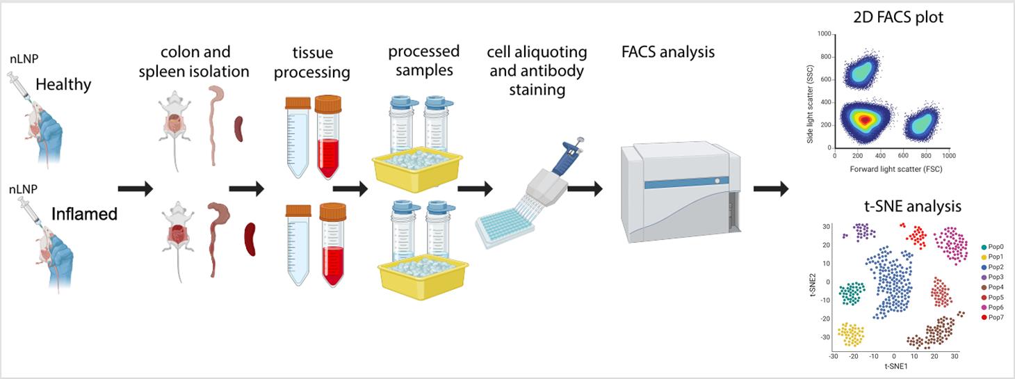
Evaluation of new lipid nanoparticle (nLNP) uptake in healthy and inflamed mouse colon using flow cytometry and t-SNE analysis. This schematic outlines the step-by-step procedure, including nLNP administration, tissue isolation and processing, antibody staining and protocol optimization, flow cytometry (FACS) data acquisition, and subsequent data analysis and validation. This image was created with BioRender.
Background
Inflammatory bowel disease (IBD), including ulcerative colitis and Crohn's disease, is characterized by chronic inflammation of the gastrointestinal (GI) tract and poses significant therapeutic challenges [1,2]. Conventional treatments often suffer from limited efficacy and significant systemic side effects due to nonspecific drug biodistribution. Lipid nanoparticles (LNPs) have emerged as a promising drug delivery platform, offering targeted delivery capability and enhanced biocompatibility [3,4]. However, assessing their cellular targets and biodistribution in the GI tract, particularly under inflammatory conditions, remains a challenge.
Existing methods for studying in vivo nanoparticle uptake, such as basic flow cytometry, provide useful insights but lack the dimensionality needed to resolve complex cellular heterogeneity. Recent advances in data analysis techniques, particularly t-distributed stochastic neighbor embedding (t-SNE), enable high-dimensional visualization and clustering, improving the identification of intricate cellular subpopulations [5,6].
This protocol builds upon previously established methods for studying nanoparticle–cell interactions by integrating t-SNE analysis into flow cytometric workflows [7]. This approach enables precise identification of colonic epithelial and macrophage populations in complex inflamed colon tissues and enhances the detection of subtle cellular patterns that traditional gating strategies may overlook. Unlike previous studies relying on single-dimensional gating, this protocol offers a robust multidimensional assessment of nanoparticle targeting and uptake.
Beyond its application to LNPs, this protocol can be adapted for other drug delivery systems, such as polymeric nanoparticles or exosomes, and in various disease models. Additionally, the integration of t-SNE into flow cytometry establishes a framework for studying cellular heterogeneity in other inflamed or complex tissues, such as respiratory epithelia. By addressing key limitations of traditional methodologies, this protocol advances nanoparticle drug delivery research and provides a powerful tool for exploring in vivo targeting mechanisms of nanoparticles.
Materials and reagents
Biological materials
1. C57BL/6J mice (Jackson Laboratory, female, 6–7 weeks of age)
Reagents
1. DAPI (Thermo Fisher Scientific, catalog number: 62247)
2. PBS (Corning, catalog number: 21-040-CV)
3. FBS (R&D Systems, catalog number: S11150H)
4. Sodium azide (Teknova, catalog number: S0209)
5. LIVE/DEAD Fixable Near IR Viability kit (Thermo Fisher Scientific, catalog number: L34982)
6. HBSS (Cytiva, catalog number: SH3058801)
7. ACK lysing buffer (Thermo Fisher Scientific, catalog number A1049201)
8. RPMI (Thermo Fisher Scientific, catalog number: 11875119)
9. CD45 (Alexa Fluor 700, clone: 30-F11, dilution: 1:800) (Thermo Fisher Scientific, catalog number: 56-045180)
10. EpCAM (APC-eFluor 780, clone: G8.8, dilution: 1:300) (Thermo Fisher Scientific, catalog number: 47-579181)
11. Ly6C (BV 650, clone: HK1.4, dilution: 1:1,000) (BioLegend, catalog number: 128049)
12. CD11b (BV 780, clone: M1/70, dilution: 1:200) (BioLegend, catalog number: 101243)
13. F4/80 (APC, clone: BM8, dilution: 1:100) (Thermo Fisher Scientific, catalog number: 17-4801-82)
14. 2.4G2 (unconjugated, clone: 2.4G2, dilution: 1:100) (BioXcell, catalog number: BE0307)
15. Dextran sulfate sodium salt (DSS), colitis grade (molecular weight: 36,000–50,000 Da) (MP Biomedicals, catalog number: 0216011090)
16. EDTA (0.5 M, pH 8.0) (Invitrogen, catalog number: AM9260G)
17. Trypan blue, 0.4% (Thermo Fisher Scientific, catalog number: T10282)
18. TrypLE [+] phenol red (Gibco, Thermo Fisher Scientific, catalog number: 12605010)
Laboratory supplies
1. 96-well, round-bottom plates (Corning, catalog number: 3797)
2. Cell strainer, pore size 100 μm, sterile (Corning, catalog number: CLS352360)
3. Cell strainer, pore size 40 μm, sterile (Corning, catalog number: CLS431750)
Equipment
1. Cytoflex LX flow cytometer (Beckman Coulter, N3-V5-B3-Y5-R3-I2, 2-parameter system equipped with 6 lasers: 375, 405, 488, 561, 638, 808 nm)
2. Automated cell counter (Invitrogen, model: Countess 3 FL)
3. Centrifuge (Eppendorf, model: 5810R)
Software and datasets
1. FlowJo (v10.10.0; BD)
2. Prism (v10.1.2; GraphPad)
3. BioRender (https://www.biorender.com/)
Procedure
Note: See Graphical overview for the general workflow.
A. Colitis induction and cell isolation from mouse tissues
1. Induce colitis in mice by administering 2% (w/v) DSS (molecular weight: 36,000–50,000 Da) in drinking water for 7 consecutive days, as described in our previously published paper [7]. Monitor mice daily for weight loss, stool consistency, and signs of rectal bleeding. Mice losing more than 15% of their initial body weight or showing severe clinical symptoms should be humanely euthanized according to approved IACUC protocols. Each experiment includes at least three mice per group (healthy, inflamed) and per repetition (n = 2–3). Mice at the same age (6–7 weeks) are acclimated for one week after purchase from the vendor.
Note: Intestinal microbiota plays a key role in host immunity and colitis—it is advisable to use the same source of animals, preferably acclimating for several days to conditions in the researcher’s animal facility.
2. Prepare nLNP and administer to mice via oral gavage (see details in [7]).
Note: It is critical to follow our published protocol; a good administration technique is crucial for proper intragastric delivery.
3. After the treatment, euthanize the mice according to approved IACUC protocols and collect the gastrointestinal (GI) tract.
4. Isolate cells from the colonic lamina propria (cLP) and colonic epithelium following the methodology described in [8]. Briefly:
a. Harvest colons from healthy and DSS-treated mice, clean, cut longitudinally, and wash with ice-cold HBSS to remove fecal material. Cut the tissue into ~2 cm segments and keep on ice until further processing.
b. For crypt isolation, incubate colon segments in epithelial cell solution [8] at 37 °C for 15 min and shake the tubes every 5 min. Place on ice for 10 min, then transfer tissue to a new 50 mL tube with 15 mL of fresh HBSS and shake vigorously. Assess a small supernatant sample under the microscope for colon crypts. If observed, proceed and filter the supernatant through a 100 μm cell strainer. Centrifuge the supernatant at 400× g for 5 min and resuspend the crypt pellet in epithelial wash buffer [8]. Keep the samples on ice until proceeding with epithelial fraction digestion.
c. For lamina propria isolation, wash the remaining tissue with HBSS, cut into ~0.5 cm pieces, and incubate in lamina propria solution [8] at 37 °C for 20 min. Perform mechanical dissociation using a pipette and repeat until fully digested. Stop digestion by adding 1 mL of FBS and 80 μL of EDTA, filter through a 40 μm cell strainer, and centrifuge at 400× g for 10 min. Resuspend the cell pellet in 2 mL of fresh RPMI. Assess the cell count and viability with 0.4% trypan blue and a cell counter.
d. Centrifuge the epithelial fraction (containing crypts) at 400× g for 5 min, then resuspend the crypt pellet with 5 mL of prewarmed TrypLE containing DNase I (100 μg/mL). Gently pipette to dissolve the pellet and incubate at room temperature (RT) for 5 min. Pipette again using a 1 mL pipette for 10 min, alternating samples every 2–3 min. If clumps persist, continue pipetting for an additional 5 min. To stop the reaction, add 1 mL of FBS, then filter the suspension through a 40μm strainer and bring the volume to 50 mL with epithelial wash buffer. Centrifuge at 400× g for 10min at 4°C; if no pellet forms, increase to 800× g. Resuspend the resulting cell pellet in 2mL of epithelial wash buffer. Determine cell count and viability using 4% trypan blue and a cell counter.
e. Validate the identity of isolated cells by flow cytometry, identifying epithelial cells as EpCAM+, lamina propria immune cells as CD45+, and macrophages as CD45+CD11b+.
5. Isolate cells from the spleens by following the procedure below.
a. Excise the spleen and disrupt it through a 40 μm cell strainer into HBSS/1% FBS buffer.
b. Centrifuge at 500× g for 5 min and remove the buffer.
c. Resuspend the pellet in 1 mL of ACK lysing buffer and incubate for 5 min at RT to lyse erythrocytes.
d. Centrifuge at 500× g for 5 min and remove the buffer.
e. Resuspend the pellet in 10 mL of HBSS buffer.
f. Centrifuge at 500× g for 5 min and remove the buffer.
g. Resuspend the pellet in 10 mL of HBSS/1% (v/v) FBS/1 mM EDTA buffer and filter through a 40 μm cell strainer.
h. Count the cells and store them on ice until use.
Notes:
1. The spleen is used for compensation controls and to demonstrate the exclusive presence of nLNP in the colon but not in peripheral tissues (Figure 1). Lymph nodes (LN) or thymus (Th) can also be used as alternatives. For more information, refer to Section D.
2. EDTA in the buffer prevents cell clumping.
3. Isolated cells can be stored in the refrigerator for up to 3 days (spleen) or overnight (colonic lamina propria and epithelium) without any noticeable loss of viability. If long-term storage is required, cells can be cryopreserved at -70 °C in RPMI/10% (v/v) FBS/10% (v/v) DMSO or a commercial freezing medium.
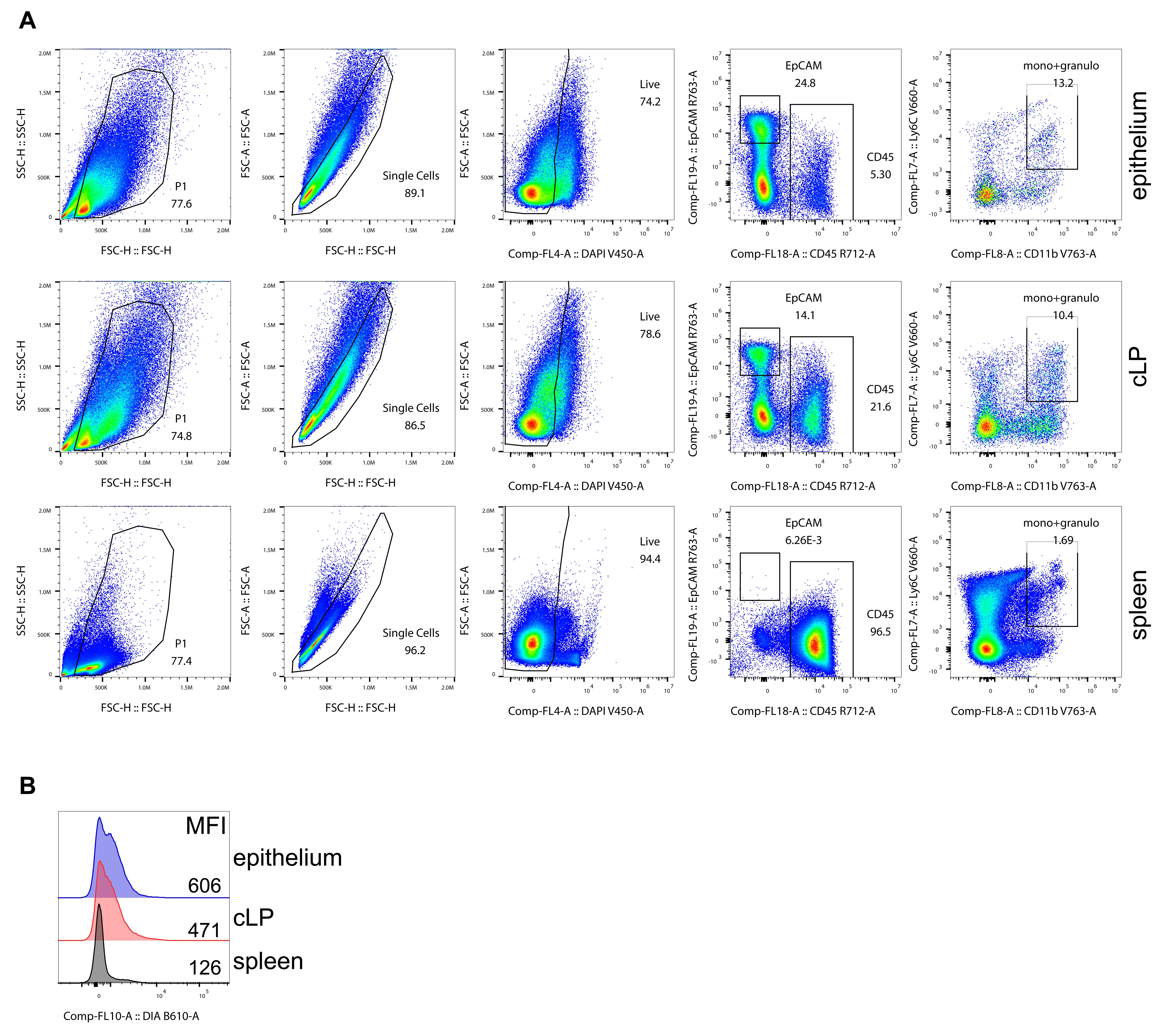
Figure 1. Gating strategy. (A) Steps for proper gating of the FACS data. (B) Nanoparticle distribution. New lipid nanoparticles (nLNPs) are exclusively found in the colon [colonic lamina propria (cLP) and colonic epithelium] and not in peripheral organs such as the spleen. Mean fluorescence intensities (MFI) are shown in gated live cells, including mono+granulo-monocytic and granulocytic myeloid CD11b+ cells, in the indicated organs.
B. Flow cytometry (FACS) staining
1. Prepare the target cells of interest and plate up to 2 × 10⁶ cells per well in a 96-well round-bottom plate. Include wells for controls (i.e., unstained cells) to set up gates for FACS analysis.
2. Centrifuge at 500× g for 1 min and aspirate the supernatant.
3. Block Fc receptors (CD16/CD32) by adding 5–10 μL of 2.4G2 antibody (at optimal concentration, e.g., 1:100) to each well and incubate at RT for 10 min to minimize nonspecific antibody binding.
4. Stain cell-surface antigens by adding 5–10 μL of the antibody mix to each well. Incubate the plate at room temperature in the dark for 10–20 min.
Notes:
1. Calculate the volume of each antibody based on its optimal concentration determined during titration and prepare the antibody mix in FACS buffer [7].
2. Unused antibody mix can be stored in the refrigerator for an extended period.
5. Wash the cells 1–2 times with 200 μL of PBS buffer, centrifuge at 500× g for 1 min, and aspirate the supernatant.
6. Resuspend the cell pellet in 200 μL of FACS buffer [7].
Note: For optimal results, analyze the cells on the flow cytometer as soon as possible. Same-day analysis is highly recommended. However, if immediate analysis is not feasible, samples can be fixed at this stage and stored in the refrigerator for up to 7 days. If fixation is necessary, follow these steps:
1. Use a fixable viability dye, such as LIVE/DEAD Fixable Near IR, to identify dead cells since fixation makes DAPI unsuitable for distinguishing between live and dead cells. Optimize the dye concentration (typically 1:500–1:1,000). For the labeling, wash cells with PBS buffer to remove serum, resuspend the pellet in 10 μL of LIVE/DEAD Fixable dye, and incubate for 10 min in the dark at RT.
2. Wash the cells once with PBS buffer, then incubate them in 10 μL/well of the diluted dye for 5–10 min at RT in the dark. Wash the cells again with PBS buffer to remove unbound dye.
3. Fix the cells by adding 100–200 μL/well of diluted Fixation/Permeabilization Solution True-Nuclear Transcription Factor Buffer Set. Pipette cells up and down with a multichannel pipette and incubate in the dark at RT for 3–5 min.
4. Centrifuge at 800× g for 3–5 min, aspirate the supernatant, and resuspend the pellet in 200 μL of PBS buffer. Wrap the plate in parafilm and store it in the refrigerator at 4 °C until the scheduled time for analysis.
5. On the day of analysis, centrifuge at 800× g for 3–5 min, aspirate the supernatant, and resuspend in 200 μL of FACS buffer. Run the samples on a flow cytometer.
7. Add DAPI (50–100 ng/mL), run on a flow cytometer, and analyze. Acquire 1 × 10⁵ live cells (ideally, acquire the same number of live cells for all the samples).
C. Antibody titration
1. Spin the antibody vial at 16,000× g for 1–2 min.
2. Prepare antibody dilution in FACS buffer (1:200, 1:400, 1:600, 1:800, 1:1,000).
Note: In rare cases, antibodies may require higher concentrations (e.g., 1:50 or 1:100). Negative staining with an antibody at 1:200 should be verified with a 1:50 stain. If issues persist, consult the supplier.
3. Plate 1 × 10⁶ cells/well, spin at 500× g for 1 min, and aspirate supernatant.
4. Resuspend the cell pellet in each antibody dilution. Leave one well unstained (resuspend in the FACS buffer).
5. Incubate for 10–20 min at RT in the dark [or at the conditions (i.e., 30 min on ice) planned to be used in the experiment].
6. Wash cells 1–2 times with 200 μL of PBS buffer, spin at 500× g for 1 min, and aspirate supernatant.
7. Resuspend the cell pellet in 200 μL of FACS buffer.
8. Run on a flow cytometer and analyze.
Notes:
1. Select fluorochromes with minimal or no spectral spillover whenever possible. For example, use FITC and APC instead of FITC and PE to reduce overlap.
2. Utilize a flow cytometer equipped with multiple lasers to assign each fluorochrome to a separate laser or laser/channel combination. For instance, in this study, the following fluorochromes were used (excitation/emission): DAPI: NUV (375/461 nm); DQ1: Blue (488/519 nm); Ly6C: BV 650 (Violet, 450/650 nm); CD11b: BV 780 (Violet, 450/785 nm); EpCAM: APC-eFluor 780 (Red, 638/750 nm); CD45: Alexa Fluor 700 (Red, 638/700 nm).
3. Perform staining at RT for 10 min to save time. However, optimal staining can be achieved by incubating for 30 min on ice to prevent understaining or staining artifacts (e.g., smears between negative and positive populations). This should be tested for each antibody batch.
D. Fluorochrome compensation
1. To minimize spectral spillover when using multiple fluorochromes, use non-overlapping fluorochromes and flow cytometers equipped with multiple lasers. For titration and compensation controls, lymphoid tissues such as the spleen, lymph nodes, or thymus are recommended, as they provide sufficient cells for accurate and reliable results.
Note: When using thymus tissue for controls, note that most thymocytes (>90%) express CD4. To make an adequate compensation sample, mix the stained thymocytes with unstained cells at a 1:1 ratio after the last wash (50% of CD4-positive cells will be used to assign the positive signal from the fluorochrome).
2. Prepare antibody dilutions for each fluorochrome used in the study. If some populations are sparse (e.g., CD11c dendritic cells in the spleen or colon), substitute the fluorochrome-conjugated antibody with anti-CD4 antibodies (or any available target expressed on a high number of cells in the lymphoid tissue, such as CD8 or B220) conjugated to the same fluorochromes. For example, use CD4-BV785 and CD4-Alexa Fluor 750 to replace CD11b-BV785 and EpCAM-Alexa Fluor 750 for compensation.
3. To prepare dead cell dye controls (e.g., DAPI), heat-kill 0.5 × 10⁶ cells by incubating them at 75 °C for 5–10 min. Cool the cells on ice for 5 min, then mix them with 0.5 × 10⁶ live cells. Add DAPI to the mixture, resulting in 50% DAPI-positive cells. Alternatively, use a fluorochrome like CD4-BV421 or CD4-eFluor450 that emits light in the same channel as DAPI.
Note: The difference between these dyes and DAPI is not substantial, but ideally, killed cells stained with DAPI should be used.
4. Prepare enough wells to include one well for each fluorochrome being tested, ensuring one unstained well is included as a control.
5. Stain the cells in each well as indicated above.
6. Run the Compensation control option in the flow cytometer’s software. Follow all steps and use the automatic compensation calculation to prepare the compensation matrix. Save the matrix to be applied to the analyzed samples.
Note: While the compensation matrix can often be reused with minimal adjustments in subsequent experiments, it is recommended that a new matrix be generated for each experiment. This accounts for minor shifts in the flow cytometer’s optical parameters over time.
E. FACS data analysis
1. Use FlowJo v10 for data analysis. The process involves using FlowJo plugins (https://www.flowjo.com/exchange/#/), which need to be downloaded to the FlowJo folder. Additionally, download R (https://cran.r-project.org/bin/windows/base/) and indicate in FlowJo its pathway (Figure 2A).
Note: This section outlines the steps for analyzing FACS data using FlowJo v10. Deviations might be necessary, but this analysis will be true for most of the data [9–11].
2. Clean data. For that purpose, prepare the sample as described in Figure 1. Begin by gating cells based on size and complexity using forward scatter (FSC) and side scatter (SSC) parameters. Next, identify and gate single cells by plotting FSC-H vs. FSC-A. Remove dead cells using DAPI or a fixable viability dye. Ensure the data is free from artifacts and smears by utilizing FlowJo plugins such as FlowClean and/or FlowAI (Workspace/Plugins; Figure 2B). Although this step is usually done manually, using plugins speeds up the process, especially when numerous parameters are analyzed.
Select all populations created in step E2 and apply the analysis across all samples by using the all samples option. Save the resulting file.
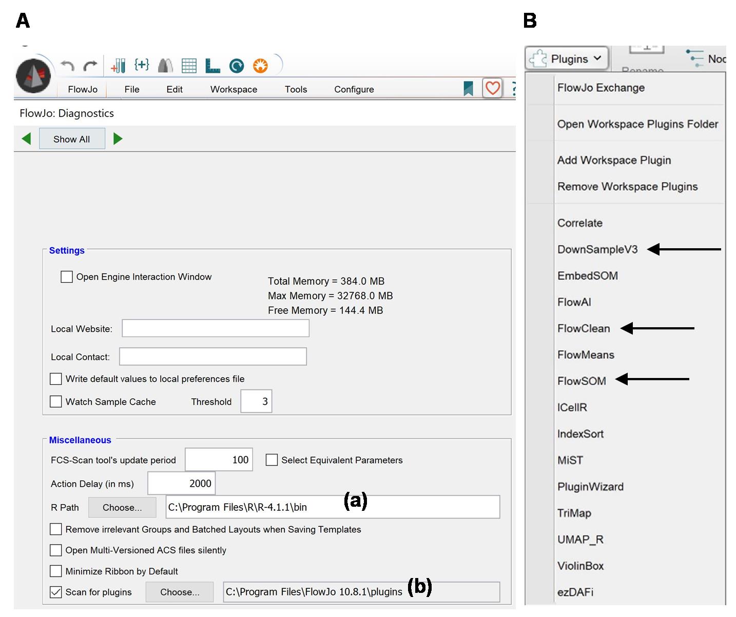
Figure 2. FlowJo Interface. (A) Workspace of FlowJo v10 showing R (a) and plugins (b) pathways. (B) Plugins available in FlowJo V10, with arrows indicating DownSampleV3, FlowClean, and FlowSOM.
3. Click on the live cell populations (or one from a given sample, then right-click and choose the option Select Equivalent Nodes, which will highlight all the live populations in all samples). Click Export/Concatenate Populations and choose Export. Click All compensated parameters and OK. This will create another workspace with all the live populations. Review the samples for any artifacts and then save the file.
4. Even when all samples recorded the same number of live events, steps E2–4 might change these numbers. Using the plugin DownSampleV3 will make the numbers even. Save the file.
5. Make a standard 2D plot analysis (Figure 3), following these steps:
a. When analyzing a small number of parameters, utilizing FlowJo plugins such as FlowMeans can help expedite the process.
b. Prepare 2D plots of all possible combinations (or the ones needed for the analysis) for one sample. Highlight the created populations and move over all samples. Save the file.
c. Using the Layout editor, move all created populations from one sample. Arrange if necessary. Hit “+” to create another layout with all the populations for all the samples. Save the file.
d. Export the picture (e.g., as .svg for easy handling in Adobe Illustrator). All the populations can be exported into an Excel file [create the table using the Table Editor option, move over all the populations from one sample, and create a file (the file will contain all samples)], which can be analyzed there or in other software like Prism.
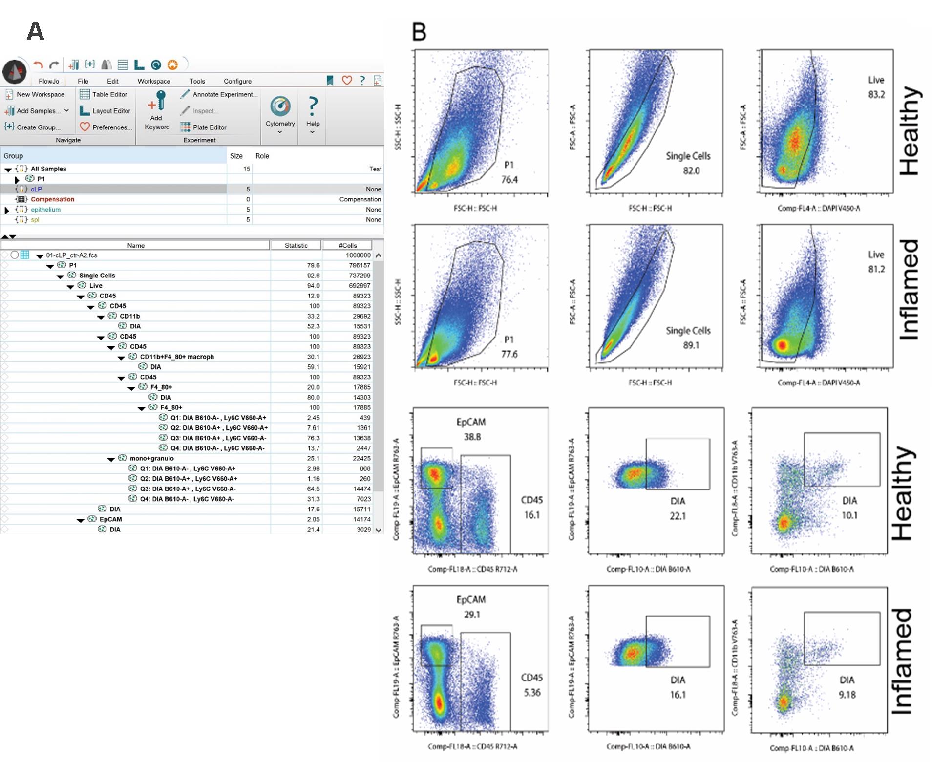
Figure 3. Conventional FACS analysis. (A) FlowJo workspace indicating all analyzed populations. (B) Example of 2D FACs plot analysis of healthy and inflamed colonic lamina propria (cLP).
6. To make t-SNE analysis, first, all samples need to be concatenated. Use the concatenate option (right mouse button, select Export/Concatenate Populations) in FlowJo (Figure 4). This will generate an additional workspace with one sample being a sum of all events from all samples. Save the file.
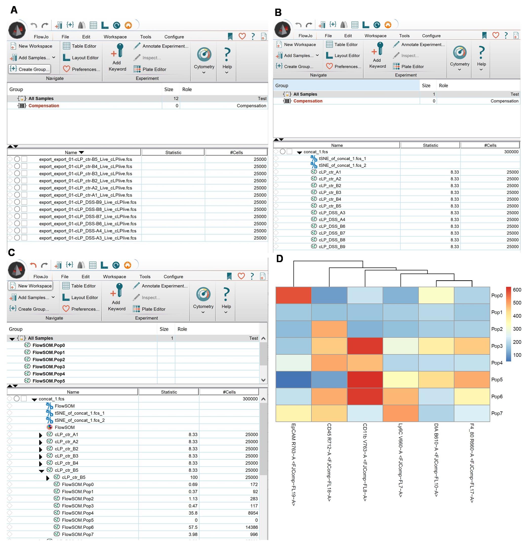
Figure 4. t-distributed stochastic neighbor embedding (t-SNE) analysis. (A) Sample numbers were normalized with DownSample plugin. (B) t-SNE was run for the concatenated file. (C) FlowSOM analysis was done for the concatenated file. (D) Heatmap generated by FlowSOM.
Notes:
1. This protocol uses t-SNE, a multi-parameter analysis method that visualizes antigen combinations in a single plot [5,12–15]. While t-SNE facilitates global analysis, data should also be validated using traditional 2D FACS analysis to confirm key findings. For example, the level of expression of a given tested antigen (MFI, mean fluorescence intensity) can be viewed in t-SNE analysis as many different populations, and the inspection of a 2D FACS plot could be used for t-SNE re-analysis to reduce the number of parameters/populations the algorithm takes into consideration. Analysis of FACS data using the machine-learning methods presented here (t-SNE and FlowSOM) have some limitations: (1) the results are sensitive to parameters such as learning rate and number of iterations; (2) t-SNE preserves local relationships but often distorts global distances; (3) a “batch effect” can alter clustering patterns; and (4) due to the stochastic nature and probabilistic process, different runs may produce slightly different results. To minimize these limitations, it is advised to (1) perform at least two separate runs to confirm the clustering pattern, (2) perform a traditional (2D) FACS analysis described above and compare with t-SNE clusters, and (3) perform UMAP analysis, which provides similar dimensionality reduction and preserves local and global structure (see below).
2. Other methods, such as UMAP, can also be employed for multi-dimensional data analysis using FlowJo plugins [16–19].
3. This section outlines the steps for analyzing FACS data using FlowJo v10. Deviations might be necessary, but this analysis will be true for most of the data [9–11].
7. Click on the sample and show it as a histogram. This will generate a histogram with the peaks corresponding to the samples used for the merge (in the order they were in the original workspace). Use the Range tool for each peak, naming it with the name of the original sample.
8. t-SNE will be made for one of the samples prepared above and then applied to the remaining samples (move the desired populations over to Group/All samples in the main window). Click on t-SNE option (Workspace/t-SNE) and choose the parameters to be analyzed by the algorithm (skip, for example, the fluorochrome used for marking dead cells) (Figure 4A, B).
9. Once the analysis is done, use the FlowSOM plugin, which will color-code the cell populations. The number of clusters that will be created is chosen manually (Figure 4C, D).
10. Change the x- and y-axes to t-SNE1 and tSNE2. Color the axes according to FlowSOM from a dropdown menu. Apply the FlowSOM clusters to all the analyzed samples.
11. Move the samples to the layout and show the legend (Figure 5A). To help identify the population, see the heatmap file generated by FlowSOM (Figure 4D).
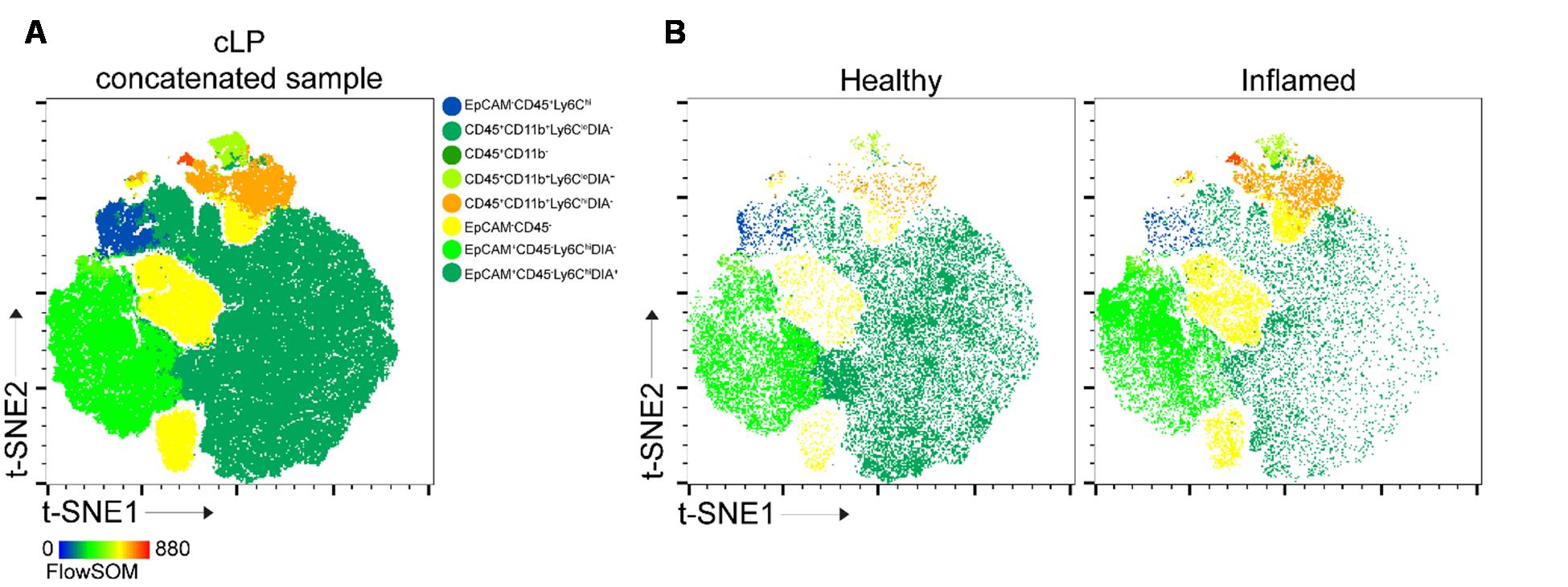
Figure 5. t-distributed stochastic neighbor embedding (t-SNE) analysis. (A) t-SNE1 vs. t-SNE2 for concatenated colonic lamina propria (cLP) sample. (B) Typical t-SNE analysis of healthy and inflamed cLP. Populations are color-coded according to FlowSOM analysis (8 populations).
Notes:
1. The EmbedSOM plugin may be used instead. Compare the default FlowJo legend with the one created by EmbedSOM.
2. t-SNE is a complex and long analysis, and it depends on the number of analyzed cells. For simplicity, one can analyze 25–50 × 103 cells/sample, which is sufficient for most analyses. If more cells are needed, one can repeat this step and increase the cell number.
3. Here, we presented 8 and 3 clusters/populations outputs generated by FlowSOM, a machine-learning model that relies on user input. The depth of the analysis depends on the researcher’s decisions, particularly regarding the interconnection between expression levels (e.g., no expression, low, mid, high) of the studied proteins (cell markers). For simplicity, we used five markers to define epithelial (EpCAM) and lymphoid (CD45) cells, as well as macrophages, monocytic, and granulocytic innate cells (CD11b, F4/80, Ly6C). Additional markers, such as those for T cells and B cells, can be included. The complexity of the analysis is dictated by the number of parameters: increasing the number of markers allows FlowSOM to incorporate protein expression levels when determining cluster numbers (see Figure 4D). Conversely, reducing the number of input parameters improves analysis speed. If an in-depth analysis is not required, or for an initial data screening, the number of populations analyzed with FlowSOM can be reduced (Figure 6). The algorithm makes sure the populations are represented as in the original file.
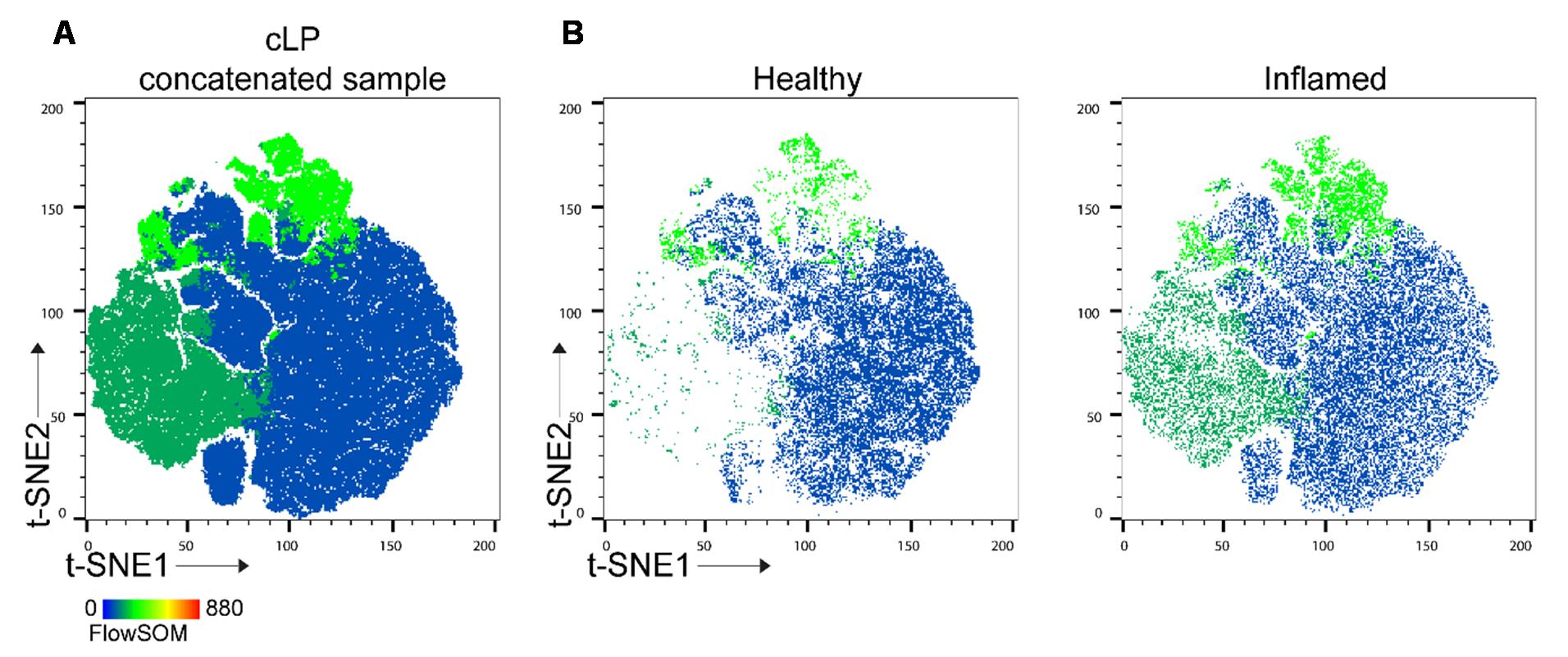
Figure 6. t-distributed stochastic neighbor embedding (t-SNE) analysis with reduced number of FlowSOM clusters. (A) t-SNE1 vs. t-SNE2 for concatenated colonic lamina propria (cLP) sample. (B) Typical t-SNE analysis of healthy and inflamed cLP.
Validation of protocol
This protocol or parts of it has been used and validated in the following research article:
• Mow et al. [7]. Harnessing a Safe Novel Lipid Nanoparticle: Targeted Oral Delivery to Colonic Epithelial and Macrophage Cells in a Colitis Mouse Model. Nanomaterials. (Figure 5A)
Acknowledgments
This work was supported by the National Institute of Diabetes and Digestive and Kidney Diseases (RO1-DK-116306 to D.M.) and the Department of Veterans Affairs (Merit Award BX002526 to D.M.). D.M. is a recipient of a Senior Research Career Scientist Award (BX004476) from the Department of Veterans Affairs. M.P.K. is a recipient of a Career Development Award (No. 833679) from the Crohn’s and Colitis Foundation of North America. The protocol described in this manuscript was developed and validated in our previous study [7].
Competing interests
The authors declare there are no conflicts of interest within the work.
References
- Fakhoury, M., Negrulj, R., Mooranian, A. and Al-Salami, H. (2014). Inflammatory Bowel Disease: Clinical Aspects and Treatments. J Inflamm Res. 7: 113–120. https://doi.org/10.2147/JIR.S65979
- Liu, D., Saikam, V., Skrada, K. A., Merlin, D., & Iyer, S. S. (2022). Inflammatory Bowel Disease Biomarkers. Med. Res. Rev. 42(5): 1856–1887. https://doi.org/10.1002/med.21893
- Yang, C., Zhang, M., Lama, S., Wang, L. and Merlin, D. (2020). Natural-Lipid Nanoparticle-Based Therapeutic Approach to Deliver 6-Shogaol and Its Metabolites M2 and M13 to the Colon to Treat Ulcerative Colitis. J Control Release. 323: 293–310. https://doi.org/10.1016/j.jconrel.2020.04.032
- Ashfaq, R., Rasul, A., Asghar, S., Kovács, A., Berkó, S. and Budai-Szűcs, M. (2023). Lipid Nanoparticles: An Effective Tool to Improve the Bioavailability of Nutraceuticals. Int J Mol Sci. 24(21). https://doi.org/10.3390/ijms242115764
- Belkina, A. C., Ciccolella, C. O., Anno, R., Halpert, R., Spidlen, J. and Snyder-Cappione, J. E. (2019). Automated Optimized Parameters for T-Distributed Stochastic Neighbor Embedding Improve Visualization and Analysis of Large Datasets. Nat Commun. 10(1): 5415. https://doi.org/10.1038/s41467-019-13055-y
- Kobak, D. and Berens, P. (2019). The Art of Using T-SNE for Single-Cell Transcriptomics. Nat Commun. 10(1): 5416. https://doi.org/10.1038/s41467-019-13056-x
- Mow, R. J., Kuczma, M. P., Shi, X., Mani, S., Merlin, D. and Yang, C. (2024). Harnessing a Safe Novel Lipid Nanoparticle: Targeted Oral Delivery to Colonic Epithelial and Macrophage Cells in a Colitis Mouse Model. Nanomaterials. 14(22): 1800. https://doi.org/10.3390/nano14221800
- Morral, C., Ghinnagow, R., Karakasheva, T., Zhou, Y., Thadi, A., et al. (2023). Isolation of Epithelial and Stromal Cells from Colon Tissues in Homeostasis and Under Inflammatory Conditions. Bio Protoc. 13(18): e4825. https://doi.org/10.21769/BioProtoc.4825
- Voronin, D. V., Kozlova, A. A., Verkhovskii, R. A., Ermakov, A. V., Makarkin, M. A., et al. (2020). Detection of Rare Objects by Flow Cytometry: Imaging, Cell Sorting, and Deep Learning Approaches. Int J Mol Sci. 21(7): 2323. https://doi.org/10.3390/ijms21072323
- Cossarizza, A., Chang, H., Radbruch, A., Abrignani, S., Addo, R., Akdis, M., Andrä, I., Andreata, F., Annunziato, F., Arranz, E., et al. (2021). Guidelines for the use of flow cytometry and cell sorting in immunological studies (third edition). Eur J Immunol. 51(12): 2708–3145. https://doi.org/10.1002/eji.202170126
- Staats, J., Divekar, A., McCoy, J. P. and Maecker, H. T. (2019). Guidelines for Gating Flow Cytometry Data for Immunological Assays. Methods Mol Biol. 2032: 81–104. https://doi.org/10.1007/978-1-4939-9650-6_5
- Toghi Eshghi, S., Au-Yeung, A., Takahashi, C., Bolen, C. R., Nyachienga, M. N., et al. (2019). Quantitative Comparison of Conventional and T-SNE-Guided Gating Analyses. Front Immunol. 10: 1194. https://doi.org/10.3389/fimmu.2019.01194
- Acuff, N. V., & Linden, J. (2017). Using Visualization of T-Distributed Stochastic Neighbor Embedding to Identify Immune Cell Subsets in Mouse Tumors. J Immunol. 198(11): 4539–4546. https://doi.org/10.4049/jimmunol.1602077
- Lucchesi, S., Nolfi, E., Pettini, E., Pastore, G., Fiorino, F., et al. (2020). Computational Analysis of Multiparametric Flow Cytometric Data to Dissect B Cell Subsets in Vaccine Studies. Cytometry A. 97(3): 259–267. https://doi.org/10.1002/cyto.a.23922
- Soh, K. T. and Wallace, P. K. (2021). Evaluation of Measurable Residual Disease in Multiple Myeloma by Multiparametric Flow Cytometry: Current Paradigm, Guidelines, and Future Applications. Int J Lab Hematol. 43(Suppl 1): 43–53. https://doi.org/10.1111/ijlh.13562
- Roca, C. P., Burton, O. T., Neumann, J., Tareen, S., Whyte, C. E., et al. (2023). A Cross Entropy Test Allows Quantitative Statistical Comparison of T-SNE and UMAP Representations. Cell Rep Methods. 3(1): 100390. https://doi.org/10.1016/j.crmeth.2022.100390
- Huang, H., Wang, Y., Rudin, C. and Browne, E. P. (2022). Towards a Comprehensive Evaluation of Dimension Reduction Methods for Transcriptomic Data Visualization. Commun Biol. 5(1): 719. https://doi.org/10.1038/s42003-022-03628-x
- Stolarek, I., Samelak-Czajka, A., Figlerowicz, M. and Jackowiak, P. (2022). Dimensionality Reduction by UMAP for Visualizing and Aiding in Classification of Imaging Flow Cytometry Data. iScience. 25(10): 105142. https://doi.org/10.1016/j.isci.2022.105142
- Ujas, T. A., Obregon-Perko, V. and Stowe, A. M. (2023). A Guide on Analyzing Flow Cytometry Data Using Clustering Methods and Nonlinear Dimensionality Reduction (TSNE or UMAP). Methods Mol Biol. 2616: 231–249. https://doi.org/10.1007/978-1-0716-2926-0_18
Article Information
Publication history
Received: Feb 3, 2025
Accepted: Apr 8, 2025
Available online: Apr 26, 2025
Published: May 20, 2025
Copyright
© 2025 The Author(s); This is an open access article under the CC BY-NC license (https://creativecommons.org/licenses/by-nc/4.0/).
How to cite
Mow, R. J., Kuczma, M. P., Shi, X., Merlin, D. and Yang, C. (2025). Tracking Oral Nanoparticle Uptake in Mouse Gastrointestinal Tract by Fluorescent Labeling and t-SNE Flow Cytometry. Bio-protocol 15(10): e5309. DOI: 10.21769/BioProtoc.5309.
Category
Immunology > Immune cell isolation > Macrophage
Immunology > Inflammatory disorder
Cell Biology > Cell-based analysis > Flow cytometry
Do you have any questions about this protocol?
Post your question to gather feedback from the community. We will also invite the authors of this article to respond.