Reconstruction of Single-Neuron Projectomes in Mice

Equipment

1. Workstation PC [e.g., Dell, model: Intel(R) Xeon(R) W-2135 CPU @ 3.70GHz, Windows 10 Pro 64, 64 GB RAM]

2. High-performance computing cluster

Software and datasets

Software

1. Fast Neurite Tracer, https://zenodo.org/record/5981001

2. Fiji, https://fiji.sc

3. Amira, https://www.thermofisher.com/, commercial license required

4. Advanced Normalization Tools (ANTs), https://docs.itk.org/en/latest/download.html

Tools and Codes

1. All tools and codes have been deposited to GitHub: https://github.com/BiyuRen/Single_Neuron_Reconstruction

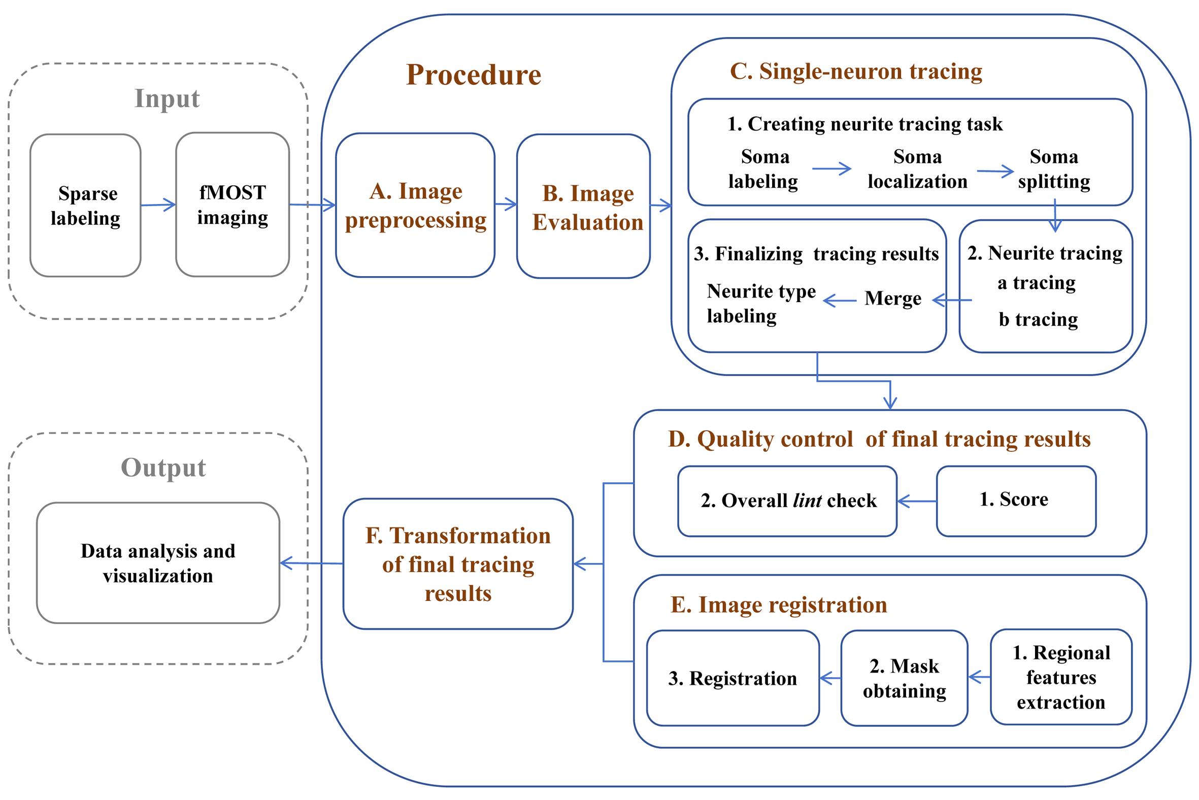
Procedure

A. fMOST image preprocessing

All mouse brain imaging samples were obtained through sparse labeling experiments and fMOST technology. The fMOST raw image data consists of two channels: the enhanced green fluorescent protein (EGFP) channel and the propidium iodide (PI) staining channel. Raw data from the two channels were preprocessed using distinct methods for specific purposes (Table 1).

1. EGFP channel: Raw data from the GFP channel were preprocessed using methods established by the FNT software developing team to generate image formats compatible with FNT software. Raw data were cut into cubes using the FNT-slice2cube command and then compressed via high-efficiency video coding (HEVC), producing image data accessible through the CH00hevc channel within FNT for single-neuron tracing. Additionally, raw data were also down-sampled to a resolution of 20 µm × 20 µm × 20 µm, accessible through the CH00DS channel within FNT for whole-brain visualization (Figure 1).

2. PI channel: The raw data from the PI channel can be preprocessed using FIJI or other image processing tools to stack multiple TIF images into a .nrrd format file (e.g., CH00PI.nrrd) for subsequent steps, including soma localization and image registration.

Table 1. Image raw data information and preprocessing

fMOST channel	Image pixel resolution	Axial resolution	Number of slices	Image preprocessing methods	Purpose
EGFP channel	0.325 × 0.325 µm	1 µm	~10,000 16-bit TIF images	FNT-slice2cube command HEVC method	CH00hevc for neurite tracing
				Down-sampling	CH00DS for overview of the whole brain
PI channel	10 × 10 µm	10 µm	~1,000 8-bit TIF images	Image stacking	CH00PI for image registration
					CH00PI for soma localization

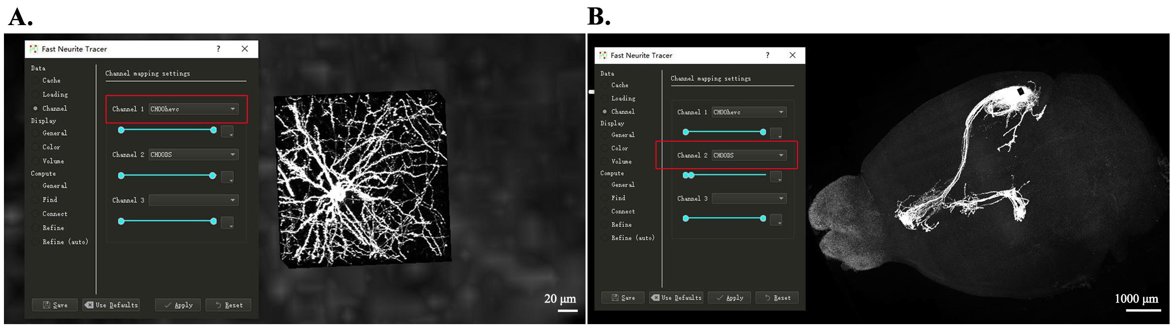
Figure 1. Image preprocessing for tracing and whole-brain visualization. (A) High-resolution image block from the CH00hevc channel in FNT, showing detailed neurite structures used for neurite tracing. (B) Down-sampled whole-brain view from the CH00DS channel in FNT, showing the entire mouse brain and facilitating global evaluation of labeling and morphology distribution.

B. Evaluation of image quality for neurite tracing

The series of brain images obtained from the previous preprocessing step would facilitate the visualization of whole-brain morphological patterns of all labeled neurons. Importantly, the overall quality of the brain images should be evaluated before proceeding with tracing in order to estimate the feasibility of performing neurite tracing at the single-cell level.

1. High-quality image examples for neurite tracing (Figure 2A)

Complete, sparse, and high signal-to-noise ratio (SNR): High-quality imaging data, characterized by completeness, sparsity, and high signal intensity, are essential for faster and more accurate tracing of single neurons.

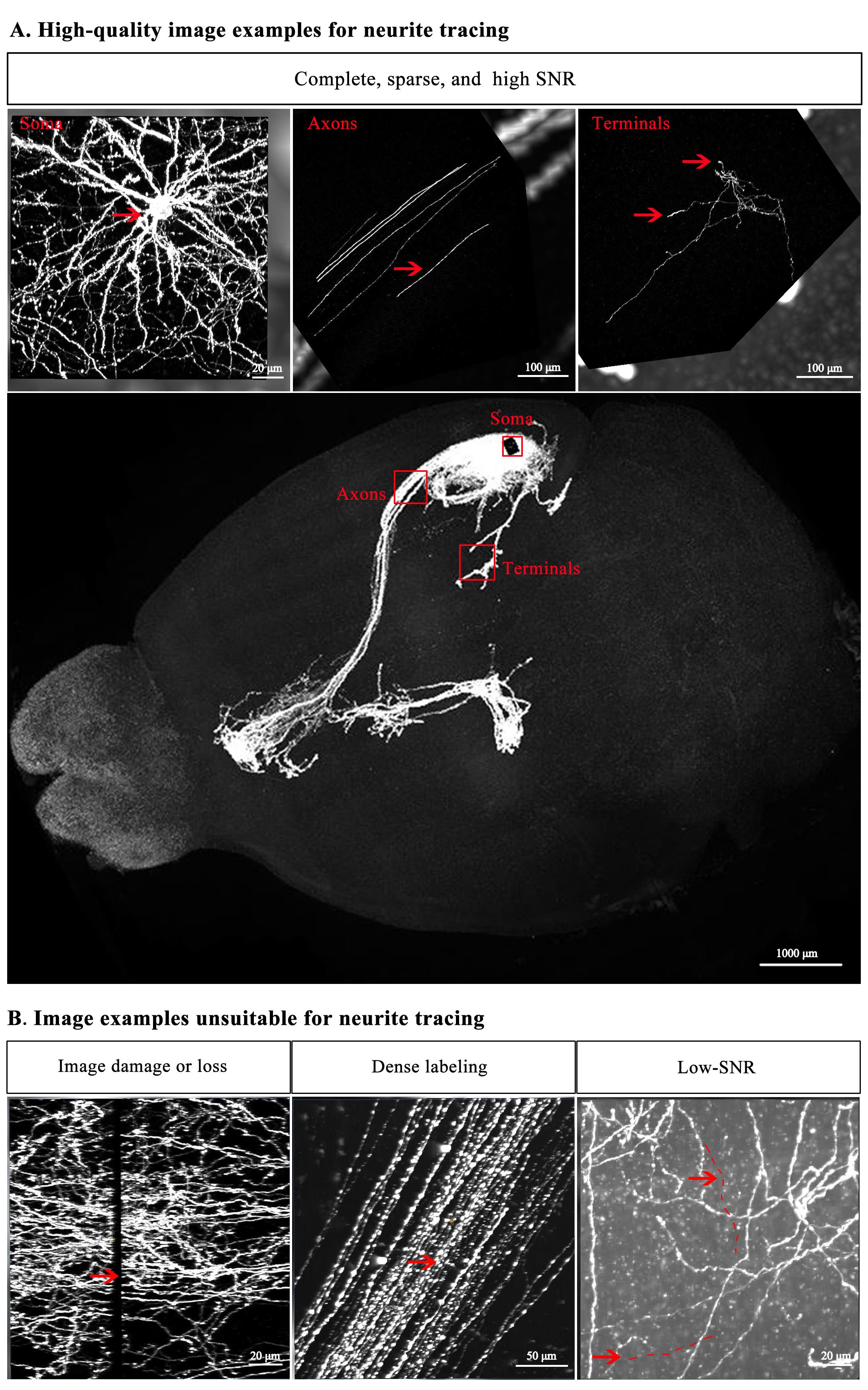
Figure 2. Representative image examples for neurite tracing. (A) neurites suitable for tracing. (B) neurites unsuitable for tracing.

2. Image examples unsuitable for neurite tracing (Figure 2B)

a. Image damage or loss: Some imaging samples may have brain areas severely damaged or lost due to improper tissue sectioning, which prevents from tracing axons that pass through these areas.

b. Dense labeling: When an excessive number of neurons are labeled in the same area, the interference among axons of individual neurons would complicate the correct tracing direction.

c. Low SNR: Weakly labeled neurons could result in unclear endpoints. High background signals would adversely dampen the integrity and accuracy of single-neuron tracing.

C. Single-neuron tracing

1. Creating a neurite tracing task in the software (Figure 3A)

a. Total soma labeling in the same mouse brain sample: Locate all labeled somas in the same sample. By creating a new neuron at the center of each soma, ultimately generate a .fnt format file (e.g., total_somas.fnt) containing information on the locations and quantities of all somas.

b. Soma localization in the targeted region: Load the file containing all soma location information and the preprocessed imaging results of the PI channel (e.g., CH00PI.nrrd) in the specified path. By using the self-developed SomaInPI tool, each soma can be mapped to its corresponding slice location, facilitating rapid determination of whether a soma is within the target brain region or not. Typically, fluorescently labeled cell bodies should be concentrated near the site of viral injection; however, due to experimental variability or varying reagent dosages, a small number of somas outside the target region may also be labeled. This step enables researchers to identify somas of interest within the target region for partial single-neuron reconstruction in the sample.

c. “Soma splitting” is to establish individual neurite tracing tasks. The file containing information on all newly created neuronal somas can be divided into multiple independent single-neuron tracing task files, allowing multiple human tracers to perform single-neuron tracing simultaneously (e.g., 001.fnt; 002.fnt...034.fnt).

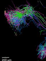
2. Neurite tracing to reconstruct the complete morphology of individual neurons (Figure 3B, C)

Human tracers responsible for neurite tracing should go through professional training to proficiently use the semi-automatic tracing software FNT, ensuring the accuracy of independently traced results as much as possible. The tracing process typically begins at the location of each neuronal soma, with careful tracing and correct connection of all branches belonging to the neuron, until the complete neuronal morphology is reconstructed.

3. Finalizing tracing results (Figure 3B, C)

a. Merging and correction: Due to the diversity and complexity of neuronal morphology, human tracers may still make errors, such as missing or adding branches. To address this issue, every neuron is traced by two independent human tracers (a and b), followed by merging and correcting the results by a third human tracer who is an experienced quality inspector. This step is essential to achieve high accuracy of the tracing results.

b. Neurite type labeling: The complete morphology of a neuron includes two distinct types of branches: dendrites and axons. In this step, neurite-type labeling is applied to differentiate between these axonal and dendritic structures in the single-neuron reconstruction (e.g., final_tracing_result.fnt), allowing for more flexible and enriched data visualization and analysis in subsequent processes.

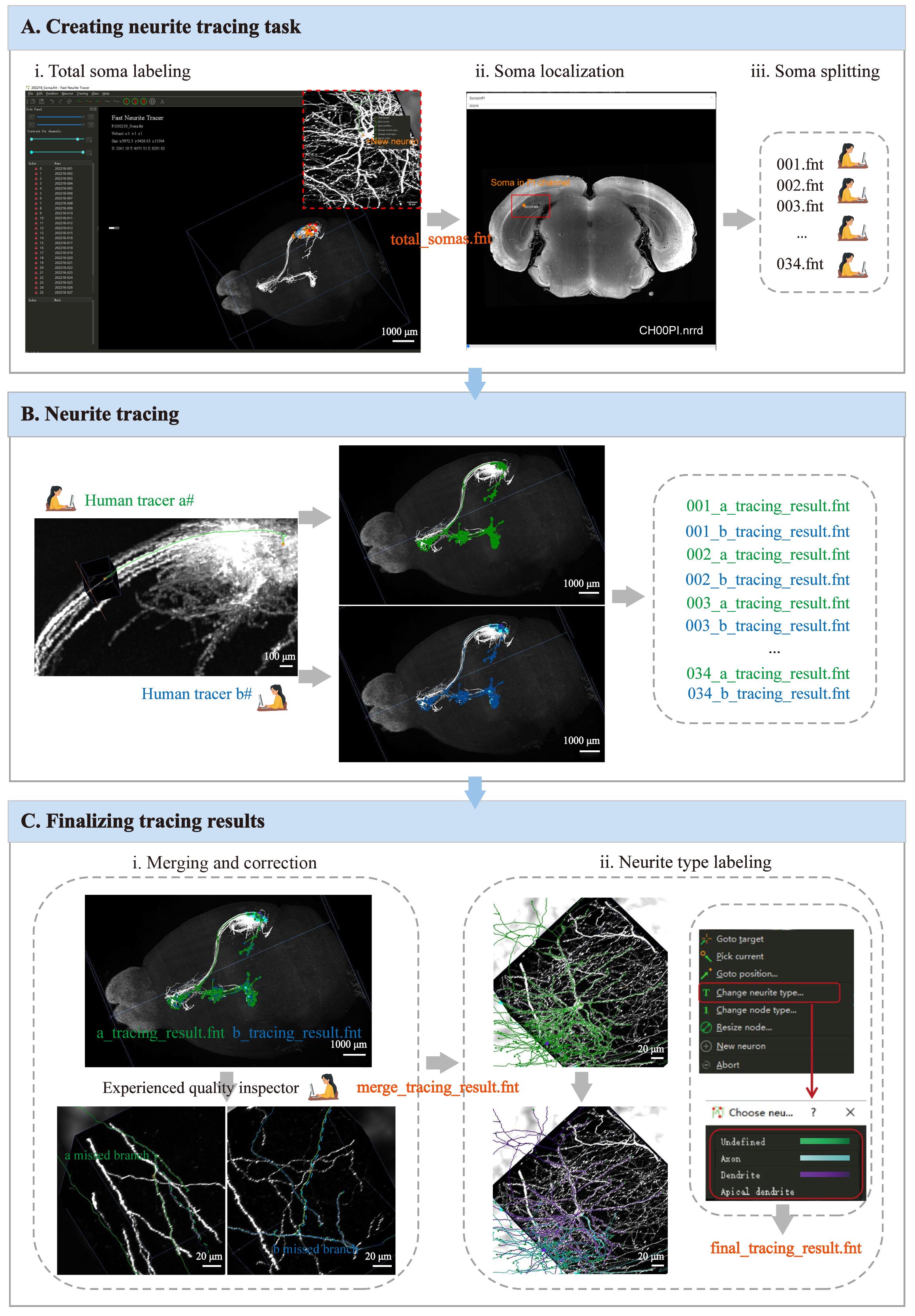
Figure 3. Procedures for single-neuron tracing. (A) Steps to create a tracing task. (B) Tracing the same neurite by two tracers. (C) Steps to merge and finalize the neurite tracing.

D. Quality control of final tracing results

1. Evaluation and scoring of traced neurons

Score: After completing all the neuron tracing tasks within the sample, the final tracing results will be reviewed and scored based on 10%–20% of the total traced neurons. The quality evaluation criteria were established based on the impact of tracing errors on the completeness and accuracy of neuronal morphology, which may affect subsequent analyses, such as those of projection regions of the brain (Table 2). Results with a score above 90 points are considered qualified, while those below 90 points are deemed unqualified and require further revisions until passing the quality control.

Table 2. Scoring criteria of traced neurons

Score	Conditions
-2	Number of false negative or false positive branches = 1
-6	Number of false negative or false positive branches = 2 or 3
-11	Number of false negative or false positive branches > 3
-11	Each miss-connection to other neurons

2. Resolving spatial conflicts between traced neurons (Figure 4A, B)

Overall lint check: The quality control steps mentioned above primarily focus on individual neuron tracing results. However, if there is mutual interference between labeled neurons within the same sample—such as overlapping, crossing, or intertwining branches—it can create ambiguity, potentially leading to trace overlap with other neurons. In such cases, we combine all tracing results from the same sample and run the lint program from the FNT software package to highlight traced branches that are in close distance (e.g., a_branches and b_branches in Figure 4B). These highlighted branches may have tracing overlap issues, which are then manually analyzed and corrected. The lint program and usage instructions are also available in our GitHub repository.

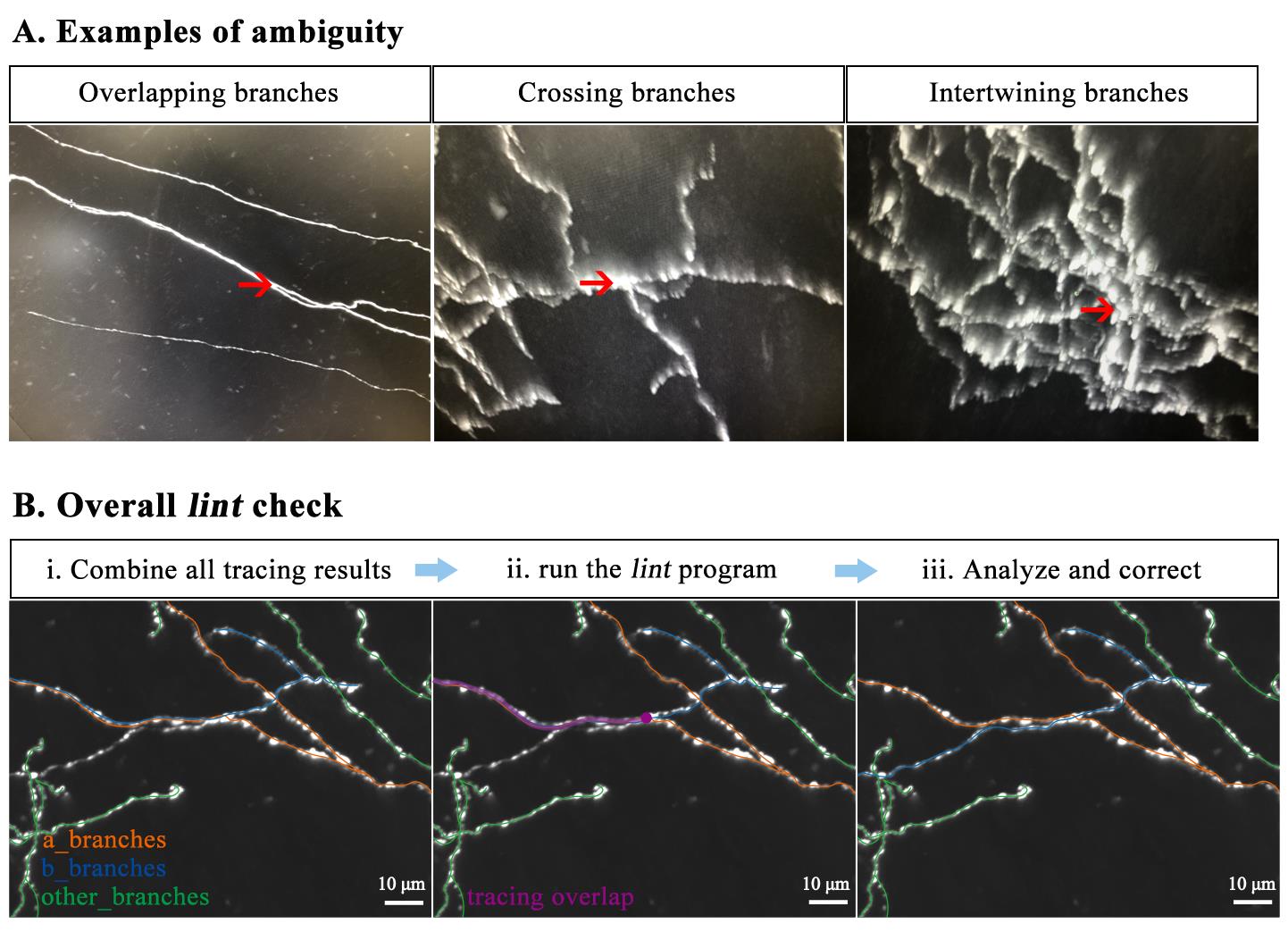
Figure 4. Resolving spatial conflicts between traced neurons by lint check. (A) Examples of fluorescent labeling leading to tracing ambiguity. (B) Steps to resolve tracing conflicts.

E. Image registration into a digital template brain

1. Regional features extraction (Figure 5A)

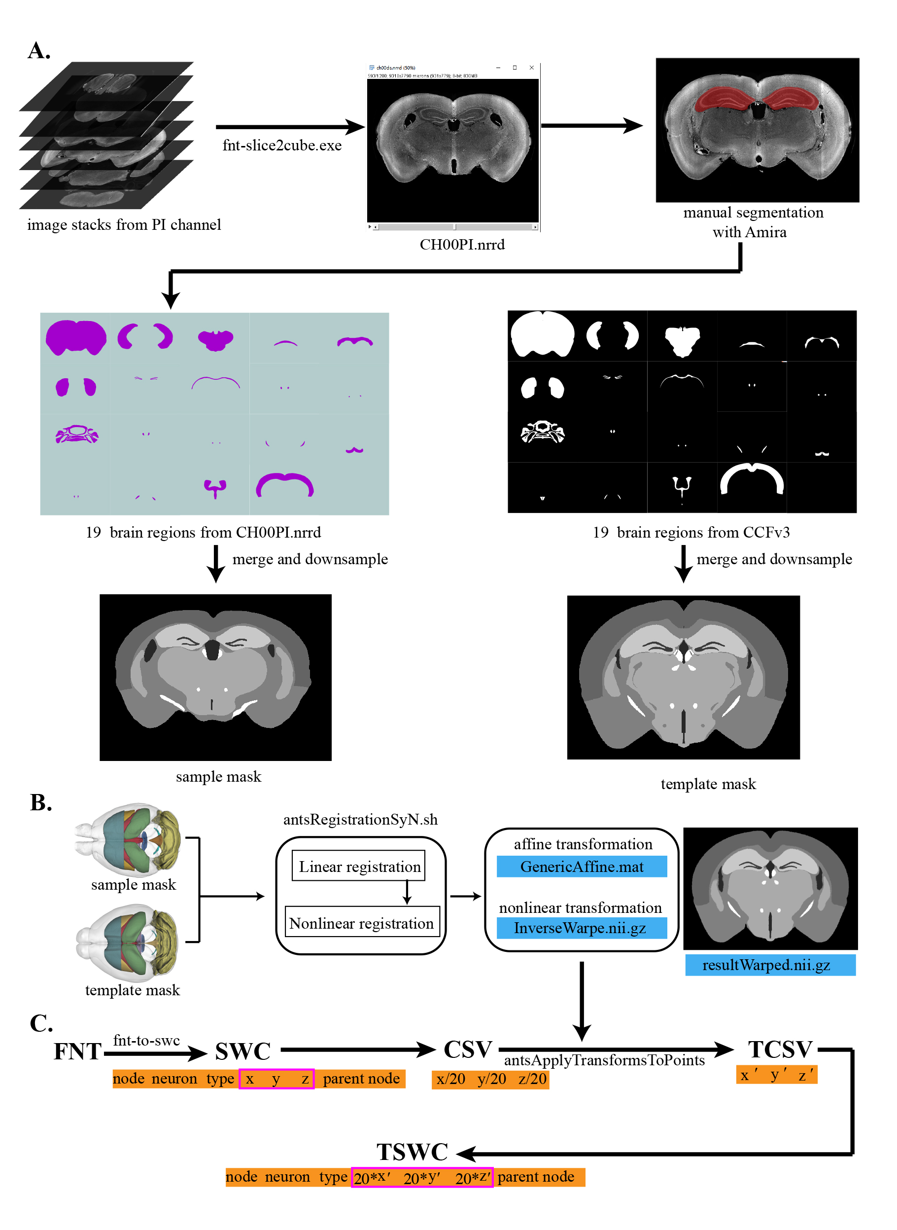
Figure 5. Image registration and neuron dataset transformation. (A) Steps to create the sample mask. (B) Steps to register the sample masks into the template mask. (C) Steps to create coordinates for dataset transformation.

a. We extract brain region features from the PI channel in the fMOST data (e.g., CH00PI.nrrd). The choice of brain regions for feature extraction determines the accuracy of registration [13]. Here, we identified the following 19 regions for feature extraction distributed in the mouse brain: whole-brain outline (Outline), isocortex (ISO), thalamus-hypothalamus (TH_HY), optic chiasm (OCH), hippocampus (HIP), anterior commissure, olfactory and temporal limbs (ACO_ACT), fourth ventricle (V4), caudate putamen (CP), dentate gyrus (DG), corpus callosum (CC), fasciculus retroflexus (FR), columns of the fornix (FX), granular layer (GR), medial habenula (MH), mammillothalamic tract (MTT), pontine gray (PG), paraventricular hypothalamic nucleus (PVH), facial nerve (VIIn) and lateral ventricle (VL). The brain regions for feature extraction typically have the following characteristics:

i. Evenly distributed throughout the brain and major brain regions.

ii. Easy to identify to ensure accuracy of feature segmentation of brain regions.

b. In order to accurately segment the above brain regions, we used an interactive segmentation tool, Amira, to perform the feature extraction procedure. The brain region features are more obvious in the coronal plane, so we typically segment the brain region in the coronal plane first and then modify the segmentation results in the sagittal plane and horizontal plane. It should be noted that when segmenting the brain region in the coronal plane, it is necessary to determine the starting and ending layers.

After the segmentation of the brain region, we can obtain 19 manually labeled brain images.

2. Sample mask and template mask for registration (Figure 5A)

a. To generate a sample mask, we merged the 19 brain regions together. During this process, the gray value parameters of these images were adjusted to a series of specific levels: 128, 100, 170, 255, 200, 255, 180, 170, 60, 255, 255, 255, 230, 255, 255, 255, 255, 60, and 40. These artificial settings of gray values were used to enhance the contrast between adjacent brain regions and facilitate the subsequent image registration process (Table 3).

b. We obtained the template mask based on the same brain regions in Allen Mouse Brain Common Coordinate Framework (CCFv3, http://brain-map.org) at 10 µm resolution [14].

Finally, sample mask and template mask were down-sampled to 20 µm resolution to improve the registration efficiency.

Table 3. Gray value parameters

Region	Outline	ISO	TH_HY	HIP	V4	CP	DG	GR	VIIn	VL	Other
Gray	128	100	170	200	180	170	60	230	60	40	255

3. Brain sample registration (Figure 5B)

We select the ANTs tools nonlinear registration method to accomplish image registration. First, the sample mask and the template mask were uploaded to a high-performance computing cluster with an ANTs-configured environment. Then, we utilized the registration command antsRegistrationSyN.sh to complete the image registration. During this process, the linear registration generated a deformation field named GenericAffine.mat, and the nonlinear registration produced a deformation field called InverseWarp.nii.gz. Neuronal or image data in the sample space can be transformed into the standard space via these two deformation fields. The resultWarped.nii.gz is the registered sample mask, which can be used to evaluate the registration effect. Scripts are provided in our GitHub repository (stepD-3-a_Registration directory).

F. Transformation of final tracing results

1. Neuron dataset transform (Figure 5C)

The final tracing results obtained in the EGFP channel will be mapped to the CCFv3 standard space. First, we used the fnt-to-SWC converter, a command tool to convert the neuron data from .fnt format to SWC format. SWC is a common format for storing neuron skeletons [15]. Each row contains seven fields for encoding the data of a single neuron: current node, neuron type, x-coordinate, y-coordinate, z-coordinate, radius, and parent node. The point where the parent node is equal to -1 is the root node. Next, we extracted x- and y-coordinates in the coronal plane, with z-coordinates determined along the anterior–posterior axis. These coordinates are then down-sampled from their original 1 µm resolution to 20 µm and stored in a CSV file. Coordinates in this CSV file are transformed into the CCFv3 standard space with the help of the deformation field and the antsApplyTransformsToPoints function in the ANTs toolkit and saved in a new CSV file (transformed CSV, TCSV). Then, we up-sample the scale of TCSV back to 1 µm and use it to update the XYZ fields of the SWC file. Finally, this updated SWC file in the standard space is called TSWC. The relevant tools and codes are provided in our GitHub repository.

Using the protocol described above, we have successfully transformed the neurons traced in the EGFP channel from its original sample space to the CCFv3 standard space. It is now ready for subsequent data analysis of single-neuron connectomes.

Validation of protocol

This protocol has been used and validated in the following research article:

1. Qiu et al. [12]. Whole-brain spatial organization of hippocampal single-neuron projectomes. Science (Figure S1, panels A–K).

Acknowledgments

This work was supported by the National Key R&D Program of China (2020YFE0205900), the National Science and Technology Innovation 2030 Major Program (2022ZD0205000), the CAS Project for Young Scientists in Basic Research (YSBR-116), the Strategic Priority Research Program of the Chinese Academy of Sciences (XDB32010105), and Lingang Lab (Grant LG202104-01-08). This protocol has been described and validated in Qiu et al [12].

Competing interests

We declare no competing interests.

References

1. Economo, M. N., Viswanathan, S., Tasic, B., Bas, E., Winnubst, J., Menon, V., Graybuck, L. T., Nguyen, T. N., Smith, K. A., Yao, Z., et al. (2018). Distinct descending motor cortex pathways and their roles in movement. Nature. 563(7729): 79–84. https://doi.org/10.1038/s41586-018-0642-9
2. Muñoz-Castañeda, R., Zingg, B., Matho, K. S., Chen, X., Wang, Q., Foster, N. N., Li, A., Narasimhan, A., Hirokawa, K. E., Huo, B., et al. (2021). Cellular anatomy of the mouse primary motor cortex. Nature. 598(7879): 159–166. https://doi.org/10.1038/s41586-021-03970-w
3. Peng, H., Xie, P., Liu, L., Kuang, X., Wang, Y., Qu, L., Gong, H., Jiang, S., Li, A., Ruan, Z., et al. (2021). Morphological diversity of single neurons in molecularly defined cell types. Nature. 598(7879): 174–181. https://doi.org/10.1038/s41586-021-03941-1
4. Winnubst, J., Bas, E., Ferreira, T. A., Wu, Z., Economo, M. N., Edson, P., Arthur, B. J., Bruns, C., Rokicki, K., Schauder, D., et al. (2019). Reconstruction of 1,000 Projection Neurons Reveals New Cell Types and Organization of Long-Range Connectivity in the Mouse Brain. Cell. 179(1): 268–281.e13. https://doi.org/10.1016/j.cell.2019.07.042
5. Lin, R., Wang, R., Yuan, J., Feng, Q., Zhou, Y., Zeng, S., Ren, M., Jiang, S., Ni, H., Zhou, C., et al. (2018). Cell-type-specific and projection-specific brain-wide reconstruction of single neurons. Nat Methods. 15(12): 1033–1036. https://doi.org/10.1038/s41592-018-0184-y
6. Sun, P., Jin, S., Tao, S., Wang, J., Li, A., Li, N., Wu, Y., Kuang, J., Liu, Y., Wang, L., et al. (2019). Highly efficient and super-bright neurocircuit tracing using vector mixing-based virus cocktail. bioRxiv: e1101/705772. https://doi.org/10.1101/705772
7. Zhong, Q., Li, A., Jin, R., Zhang, D., Li, X., Jia, X., Ding, Z., Luo, P., Zhou, C., Jiang, C., et al. (2021). High-definition imaging using line-illumination modulation microscopy. Nat Methods. 18(3): 309–315. https://doi.org/10.1038/s41592-021-01074-x
8. Harris, J. A., Mihalas, S., Hirokawa, K. E., Whitesell, J. D., Choi, H., Bernard, A., Bohn, P., Caldejon, S., Casal, L., Cho, A., et al. (2019). Hierarchical organization of cortical and thalamic connectivity. Nature. 575(7781): 195–202. https://doi.org/10.1038/s41586-019-1716-z
9. Oh, S. W., Harris, J. A., Ng, L., Winslow, B., Cain, N., Mihalas, S., Wang, Q., Lau, C., Kuan, L., Henry, A. M., et al. (2014). A mesoscale connectome of the mouse brain. Nature. 508(7495): 207–214. https://doi.org/10.1038/nature13186
10. Gao, L., Liu, S., Gou, L., Hu, Y., Liu, Y., Deng, L., Ma, D., Wang, H., Yang, Q., Chen, Z., et al. (2022). Single-neuron projectome of mouse prefrontal cortex. Nat Neurosci. 25(4): 515–529. https://doi.org/10.1038/s41593-022-01041-5
11. Li, H., Jiang, T., An, S., Xu, M., Gou, L., Ren, B., Shi, X., Wang, X., Yan, J., Yuan, J., et al. (2024). Single-neuron projectomes of mouse paraventricular hypothalamic nucleus oxytocin neurons reveal mutually exclusive projection patterns. Neuron. 112(7): 1081–1099.e7. https://doi.org/10.1016/j.neuron.2023.12.022
12. Qiu, S., Hu, Y., Huang, Y., Gao, T., Wang, X., Wang, D., Ren, B., Shi, X., Chen, Y., Wang, X., et al. (2024). Whole-brain spatial organization of hippocampal single-neuron projectomes. Science. 383(6682): eadj9198. https://doi.org/10.1126/science.adj9198
13. Ni, H., Tan, C., Feng, Z., Chen, S., Zhang, Z., Li, W., Guan, Y., Gong, H., Luo, Q., Li, A., et al. (2020). A Robust Image Registration Interface for Large Volume Brain Atlas. Sci Rep. 10(1): 2139. https://doi.org/10.1038/s41598-020-59042-y
14. Wang, Q., Ding, S. L., Li, Y., Royall, J., Feng, D., Lesnar, P., Graddis, N., Naeemi, M., Facer, B., Ho, A., et al. (2020). The Allen Mouse Brain Common Coordinate Framework: A 3D Reference Atlas. Cell. 181(4): 936–953.e20. https://doi.org/10.1016/j.cell.2020.04.007
15. Cannon, R., Turner, D., Pyapali, G. and Wheal, H. (1998). An on-line archive of reconstructed hippocampal neurons. J Neurosci Methods. 84: 49–54. https://doi.org/10.1016/s0165-0270(98)00091-0