- Protocols

- Articles and Issues
- For Authors
- About
- Become a Reviewer

ChIP-seq Data Processing and Relative and Quantitative Signal Normalization for Saccharomyces cerevisiae
(*contributed equally to this work) Published: Vol 15, Iss 9, May 5, 2025 DOI: 10.21769/BioProtoc.5299 Views: 3012
Reviewed by: Hemant Kumar PrajapatiPriyanka MittalAakanksha J. Sane
Advertisement


Protocol Collections
Comprehensive collections of detailed, peer-reviewed protocols focusing on specific topics


Related protocols
Abstract
Chromatin immunoprecipitation with high-throughput sequencing (ChIP-seq) is a widely used technique for genome-wide analyses of protein–DNA interactions. This protocol provides a guide to ChIP-seq data processing in Saccharomyces cerevisiae, with a focus on signal normalization to address data biases and enable meaningful comparisons within and between samples. Designed for researchers with minimal bioinformatics experience, it includes practical overviews and refers to scripting examples for key tasks, such as configuring computational environments, trimming and aligning reads, processing alignments, and visualizing signals. This protocol employs the sans-spike-in method for quantitative ChIP-seq (siQ-ChIP) and normalized coverage for absolute and relative comparisons of ChIP-seq data, respectively. While spike-in normalization, which is semiquantitative, is addressed for context, siQ-ChIP and normalized coverage are recommended as mathematically rigorous and reliable alternatives.
Key features
• ChIP-seq data processing workflow for Linux and macOS integrating data acquisition, trimming, alignment, processing, and multiple forms of signal computation, with a focus on reproducibility.
• ChIP-seq signal generation using siQ-ChIP to quantify absolute IP efficiency—providing a rigorous alternative to spike-in normalization—and normalized coverage for relative comparisons.
• Broad applicability demonstrated with Saccharomyces cerevisiae (experimental) and Schizosaccharomyces pombe (spike-in) data but suitable for ChIP-seq in any species.
• In-depth notes and troubleshooting guide users through setup challenges and key concepts in basic bioinformatics, data processing, and signal computation.
Keywords: BioinformaticsGraphical overview
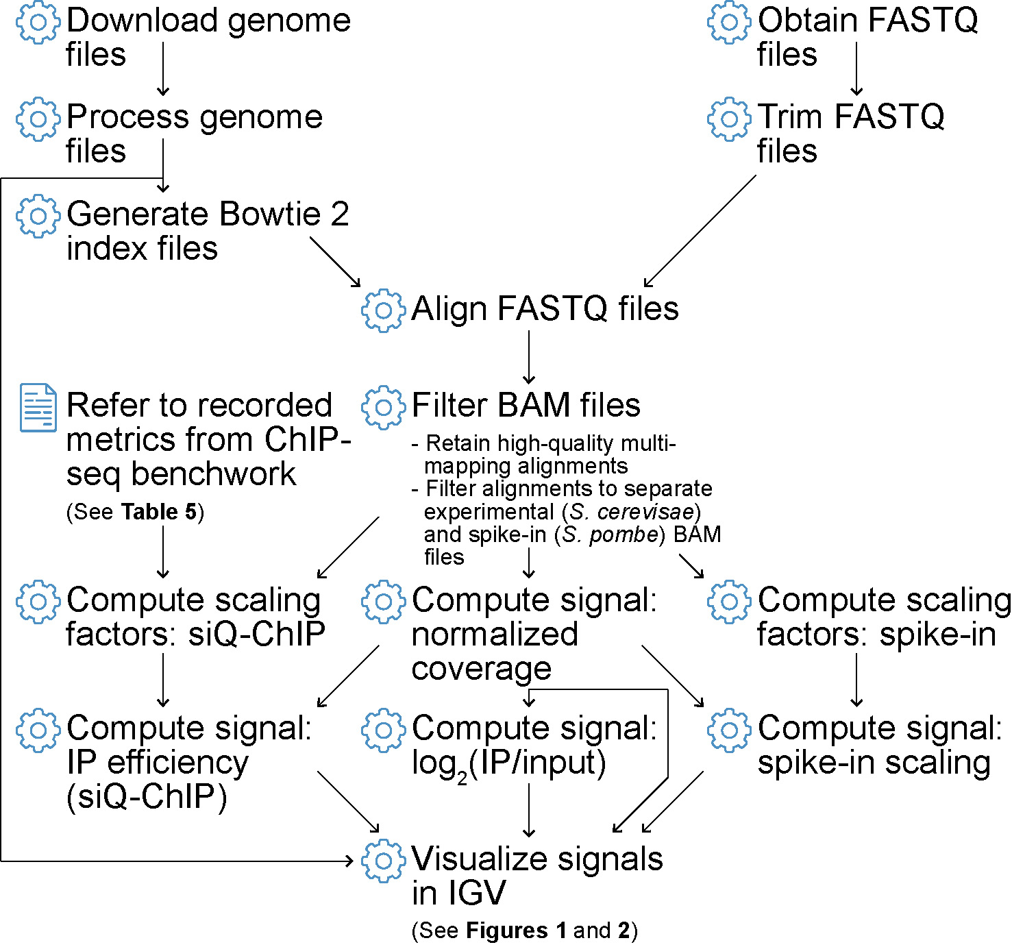
Flowchart depicting ChIP-seq data processing steps covered in this protocol
Background
Chromatin immunoprecipitation followed by high-throughput DNA sequencing (ChIP-seq) is a widely used technique for studying protein–DNA interactions across the genome [1–4]. ChIP-seq identifies regions bound by proteins such as histones, transcription factors, and other chromatin-associated factors, making it central to chromatin biology, epigenetics, and other fields. The method begins with the cross-linking of chromatin to capture DNA–protein interactions. The cross-linked chromatin is then isolated, fragmented, and immunoprecipitated using antibodies specific to the target protein. The associated DNA is recovered and sequenced with next-generation sequencing (NGS) technology. Sequenced reads (see General notes 1 and 2) are aligned to a reference genome (see General note 3) and processed into a genome-wide “signal” reflecting the frequency of protein–DNA interactions.
ChIP-seq signal, typically represented as a histogram of fragments along the genome (x-axis; see General note 4), lends itself to comparisons of protein distributions within and across samples. However, signal variability makes it difficult to link enrichment levels (y-axis) to the biological activity of proteins, particularly across different experimental conditions. Factors such as cell state, cell number, cross-linking, fragmentation, DNA amplification, library preparation, and sequencing conditions make it challenging to establish a consistent scale for comparing protein enrichment, while poor antibody specificity can further undermine accuracy [5–10].
To address this variability, researchers developed various normalization methods (see General note 5), including spike-in controls [11–15]. Spike-in normalization involves adding a known quantity of exogenous chromatin to experimental samples as a reference for signal scaling. However, evidence indicates that spike-ins often fail to reliably support comparisons within and between samples [5,16], as discussed below. The recently developed sans spike-in quantitative ChIP (siQ-ChIP) method overcomes these limitations by measuring absolute protein–DNA interactions [i.e., immunoprecipitation (IP) efficiency] genome-wide, without relying on exogenous chromatin as a reference [5,16]. Importantly, siQ-ChIP does not introduce additional experimental requirements beyond those already inherent to ChIP-seq. Rather, it explicitly highlights fundamental factors—such as antibody behavior, chromatin fragmentation, and input quantification—that influence signal interpretation, reinforcing best practices intrinsic to ChIP-seq (see General notes 6 and 7). This protocol introduces the computation of siQ-ChIP-adjusted signal for absolute, quantitative comparisons of ChIP-seq data within and between samples, as well as normalized coverage for relative comparisons [16] (see General note 8). Although steps for computing semiquantitative spike-in scaled signals are included for context [15], siQ-ChIP and normalized coverage are strongly recommended as mathematically rigorous and more effective tools for ChIP-seq analyses.
Designed for researchers with minimal bioinformatics experience (see General note 9), this protocol covers computational setup, read processing, and signal visualization. The Procedure section covers program installations and computational environment setup, while the Data analysis section provides guidance on data acquisition and processing. The protocol focuses on Saccharomyces cerevisiae and discusses data processing and signal interpretation relevant to its ribosomal DNA (rDNA) locus, a site of high biological interest [17] with specific computational considerations (see General note 10). However, the data processing methods apply to genome-wide analysis, not just the rDNA. While the examples and applications use S. cerevisiae data, the principles and processing steps are broadly applicable to ChIP-seq data from any organism, including widely studied models such as Homo sapiens and Mus musculus.
Software and datasets
A. Computational and experimental resources
This section provides an overview of the computational and experimental resources used in the protocol, including system requirements, software tools, yeast strains, reference genomes, and key experimental parameters. Table 1 lists the operating systems used for implementation and testing. Table 2 details the primary programs required to execute the workflow, along with recommended versions for compatibility. Table 3 describes the yeast strains used for ChIP-seq data generation (see General note 11), specifying their genotypes and references. This protocol uses data from an engineered system in which FLAG epitope sequences were integrated with S. cerevisiae HHO1 (histone H1) [18], S. cerevisiae HMO1 (chromatin-associated high mobility group protein), and S. pombe abp1 (ARS binding protein 1, a CENP-B homolog) [19,20], resulting in FLAG-tagged proteins. This system promotes uniform antibody affinity across endogenous (S. cerevisiae) and spike-in (S. pombe) chromatin, minimizing variability in binding efficiency (discussed in later sections and notes). All yeast strains used in this protocol are available upon request from the Tsukiyama Lab (ttsukiya@fredhutch.org). Table 4 presents the reference genomes used for read alignment and data processing. Table 5 documents ChIP-seq experimental parameters for S. cerevisiae samples, including input and IP volumes, chromatin masses, and cell cycle states, which are needed to compute siQ-ChIP α proportionality constants. ChIP-seq data are available in the Gene Expression Omnibus (GEO) via accession number GSE288548.
Table 1. Operating systems (os) and respective versions used to implement, test, and run the protocol.
| os | Version |
|---|---|
| macOS | 15.1.1 24B91 |
| Ubuntu (Linux) | 18.04.6 LTS (Bionic Beaver) |
Table 2. Programs used to implement, test, and run the protocol, excluding dependencies and libraries. The table also includes program version numbers, associated operating systems (os), and relevant references. While most program versions do not need strict adherence, the following version guidelines are recommended for compatibility: Atria [21] 4.0.0 or later, installed with Julia [22,23] 1.8.5; Bash 3.2.0 or later; GNU Parallel [24] 20150222 or later; Python [25] 3.6.0 or later.
| Program | Version | os | Reference(s) |
|---|---|---|---|
| Atria | 4.0.3 | macOS, Linux | [21] |
| Awk (GNU) | 5.3.1 | macOS, Linux | [26,27] |
| Bash | 3.2.57(1) | macOS | |
| Bash | 4.4.20(1) | Linux | |
| bc | 1.07.1 | macOS, Linux | |
| Bowtie2 | 2.5.4 | macOS, Linux | [28–30] |
| Conda | 24.7.1 | macOS, Linux | |
| Git | 2.39.5 | macOS | |
| Git | 2.17.1 | Linux | |
| IGV (“with Java Included”) | 2.19.1 | macOS | [31–34] |
| Julia | 1.8.5 | macOS, Linux | [22,23] |
| Mamba | 1.5.9 | macOS, Linux | |
| Miniforge3 | 24.7.1-2 | macOS, Linux | |
| Parallel (GNU) | 20170422 | macOS, Linux | [24] |
| Python | 3.12.7 | macOS, Linux | [25] |
| Samtools | 1.21 | macOS, Linux | [35,36] |
| SLURM | 24.05.4 | Linux | [37] |
Table 3. S. cerevisiae and S. pombe strains used for ChIP-seq data generation. “Organism” indicates whether the strain is S. cerevisiae or S. pombe. “strain_full” represents the complete strain identifier; for S. cerevisiae, that includes a three-letter prefix indicating the lab of origin (e.g., “yTT” represents “yeast Toshio Tsukiyama”). “genotype_full” specifies that the S. cerevisiae HHO1 and HMO1 genes were separately tagged with sequences encoding 3×FLAG epitopes, including flexible linkers (2L-3FLAG), generating HHO1-2L-3FLAG and HMO1-2L-3FLAG strains; and the S. pombe gene abp1 was tagged with a 3×FLAG epitope sequence, generating abp1-3FLAG. The final column lists the studies in which the strains were described. For more details, see General note 11.
| Organism | strain_full | genotype_full | Reference |
|---|---|---|---|
| Saccharomyces cerevisiae | yTT6336 | HHO1-2L-3FLAG | [18] |
| Saccharomyces cerevisiae | yTT6337 | HHO1-2L-3FLAG | [18] |
| Saccharomyces cerevisiae | yTT7750 | HMO1-2L-3FLAG | This protocol |
| Saccharomyces cerevisiae | yTT7751 | HMO1-2L-3FLAG | This protocol |
| Schizosaccharomyces pombe | Sphc821 | abp1-3FLAG | [19] |
Table 4. Species genomes used for alignment, data processing, and signal visualization. “Species” specifies whether the genome is for S. cerevisiae or S. pombe. “Genome” refers to the reference genome assembly strain/name. “Version” indicates the assembly version used. “Database” refers to the source of the genome assembly. Assembly versions do not need to be strictly followed. For more information, refer to Data analysis A, B, E, and J.
| Species | Genome | Version | Database |
|---|---|---|---|
| S. cerevisiae | S288C | R64-5-1 20240529 | Saccharomyces Genome Database |
| S. pombe | 972h- | 2024-11-01 | Pombase |
Table 5. S. cerevisiae ChIP-seq experimental parameters, including those needed to compute siQ-ChIP α proportionality constants. Parameters include input volumes (“vol_in”) and total volumes before the removal of input (“vol_all”) in microliters, as well as input and IP chromatin masses (“mass_in” and “mass_ip”) in nanograms, measured during ChIP-seq benchwork [5,16]. Average fragment lengths in base pairs (bp; “length_in” and “length_ip”) are required but do not need to be included in the table, as they can be calculated from sample BAM files during α computation (see Data analysis H). “genotype_full” and “genotype”: Genetic constitution of S. cerevisiae sample. As there is no indication that the tag compromises the function of either Hho1 or Hmo1, these strains are labeled “WT” (wild type) in filenames. “State”: Cell-cycle phase. “G1” represents cells in the first gap phase of the cell cycle, preparing for DNA synthesis. “G2/M” includes cells in the second gap phase (G2), undergoing DNA synthesis, and mitosis (M), representing the cell cycle substages leading to and including cell division. “Q” represents quiescent cells in a reversible state of cell cycle withdrawal. “Factor”: Protein immunoprecipitated using mouse monoclonal anti-FLAG M2 antibody (Sigma, F1804). “Hho1” corresponds to S. cerevisiae histone H1, and “Hmo1” to S. cerevisiae chromatin-associated high mobility group family member protein. “strain_full”: Full S. cerevisiae strain identifier. “Strain”: Abbreviated S. cerevisiae strain identifier, which may be substituted with “replicate” (or “rep”).
| genotype_full | Genotype | State | Factor | strain_full | Strain | vol_in | vol_all | mass_in | mass_ip |
|---|---|---|---|---|---|---|---|---|---|
| HHO1-2L-3FLAG | WT | G1 | Hho1 | yTT6336 | 6336 | 20 | 300 | 72.5 | 2.7 |
| HHO1-2L-3FLAG | WT | G1 | Hho1 | yTT6337 | 6337 | 20 | 300 | 81.1 | 5 |
| HHO1-2L-3FLAG | WT | G2M | Hho1 | yTT6336 | 6336 | 20 | 300 | 104.9 | 6.6 |
| HHO1-2L-3FLAG | WT | G2M | Hho1 | yTT6337 | 6337 | 20 | 300 | 85.2 | 6.1 |
| HHO1-2L-3FLAG | WT | Q | Hho1 | yTT6336 | 6336 | 20 | 300 | 72.7 | 116.9 |
| HHO1-2L-3FLAG | WT | Q | Hho1 | yTT6337 | 6337 | 20 | 300 | 69.6 | 70.6 |
| HMO1-2L-3FLAG | WT | G1 | Hmo1 | yTT7750 | 7750 | 20 | 300 | 79.9 | 8.4 |
| HMO1-2L-3FLAG | WT | G1 | Hmo1 | yTT7751 | 7751 | 20 | 300 | 63.6 | 3.2 |
| HMO1-2L-3FLAG | WT | G2M | Hmo1 | yTT7750 | 7750 | 20 | 300 | 32.4 | 5.4 |
| HMO1-2L-3FLAG | WT | G2M | Hmo1 | yTT7751 | 7751 | 20 | 300 | 93.4 | 3.4 |
| HMO1-2L-3FLAG | WT | Q | Hmo1 | yTT7750 | 7750 | 20 | 300 | 67.9 | 27.4 |
| HMO1-2L-3FLAG | WT | Q | Hmo1 | yTT7751 | 7751 | 20 | 300 | 106.6 | 14.8 |
B. Companion GitHub repository for protocol implementation
This protocol is accompanied by the GitHub repository protocol_chipseq_signal_norm (github.com/kalavattam/protocol_chipseq_signal_norm), which contains tools, scripts, and resources for implementing the workflow described in this tutorial. protocol_chipseq_signal_norm includes driver and utility scripts, functions, and a Markdown notebook, workflow.md, that provides code examples with explanatory text for the steps outlined in the Procedure and Data analysis sections. All content is organized and documented following the principles in [38,39]. Key features include the following:
• Initializing variables for directory paths, files, and computational environments, among other things.
• Defining script arguments.
• Organizing input and output files within structured directory systems.
• Validating paths, files, dependencies, etc.
• Automating experiments with driver scripts that coordinate processes like read trimming, alignment, post-processing, and signal track generation. Most driver scripts accept serialized lists (e.g., comma-delimited strings) of FASTQ, BAM, or bedGraph input files, which can be generated using the utility script find_files.sh (see General note 12).
• Parallelizing tasks on high-performance computing clusters configured to use SLURM [37] or on local or remote systems using GNU Parallel [24].
• Capturing detailed logs for all commands to support troubleshooting and reproducibility.
Additionally, the protocol_chipseq_signal_norm repository includes tab-separated value (TSV) files for downloading experimental datasets (see Data analysis C) and a TSV file with metadata and parameters required for running siQ-ChIP (see Data analysis H).
Procedure
Note: This protocol is designed for use on Linux and macOS systems with the programs, species, and resources described in Tables 1–5. It has not been tested on Windows. All code examples have been validated in Bash (see General note 13).
A. Install and configure Miniforge
Miniforge is an open-source tool for managing bioinformatics software in isolated environments—self-contained workspaces that prevent software conflicts (see General note 14). This protocol uses Miniforge to create and manage an environment, env_protocol, that contains programs for read alignment, alignment processing, signal computation, and signal visualization. If other software managers (e.g., Anaconda) are installed, it is recommended to uninstall them before installing Miniforge to avoid conflicts.
1. Determine the appropriate Miniforge installer to use.
To determine the operating system (OS) and system architecture, open a terminal (see General note 15) and use the uname command, assigning the outputs to variables:
# OS
case $(uname -s) in
Darwin) os="MacOSX" ;;
Linux) os="Linux" ;;
*) echo "Error: Unsupported operating system: '$(uname -s)'." >&2 ;;
esac
# Architecture
ar=$(uname -m) # e.g., "x86_64" for Intel/AMD, "arm64" for ARM
2. Download and install Miniforge.
Variables os and ar contain operating system (OS) and architecture system details, respectively. The installation script is downloaded to the HOME directory (see General note 16) and executed as follows:
https="https://github.com/conda-forge/miniforge/releases/latest/download"
script="Miniforge3-${os}-${ar}.sh"
cd "${HOME}"
curl -L -O "${https}/${script}"
bash "${script}"
Allow Miniforge to initialize the conda base environment automatically (see Troubleshooting 1 and 2).
3. Configure the Miniforge channels.
Edit the .condarc file to prioritize conda-forge and bioconda channels (see Troubleshooting 3):
channels:
- conda-forge
- bioconda
channel_priority: flexible
B. Clone the protocol repository and install the project environment
After configuring Miniforge, use Git to clone the protocol repository, protocol_chipseq_signal_norm (see General notes 17 and 18 and Troubleshooting 4). Then, use its script install_envs.sh to set up env_protocol, the project environment.
1. Clone the repository.
In this protocol, all cloned repositories are stored in a dedicated repos subdirectory under the HOME directory:
mkdir -p "${HOME}/repos"
cd "${HOME}/repos"
Clone the repository and navigate to it:
git clone "https://github.com/kalavattam/protocol_chipseq_signal_norm.git"
cd "protocol_chipseq_signal_norm"
2. Install the environment with install_envs.sh.
Run the following command to create and install the required environment:
bash "scripts/install_envs.sh" --env_nam "env_protocol" --yes
C. Install and configure Atria for FASTQ adapter and quality trimming
To promote accurate alignment of sequenced reads, it is important to remove adapter sequences and low-quality base calls from FASTQ files. For this, we use Atria [21], a tool written in Julia [22,23] that excels in adapter and quality trimming. Follow these steps to install and configure Atria:
1. Install Julia.
Download Julia 1.8.5 as a pre-compiled tarball (see General notes 19 and 20) for the appropriate OS and system architecture. Retrieve the tarball from the official Julia website, saving it to the HOME directory (see General note 16). Be sure to select the correct values for the following variables:
• os: Operating system (“mac” for macOS, “linux” for Linux, etc.)
• ar_s: Short architecture name (“aarch64” for ARM, “x64” for x86_64, etc.)
• ar_l: Long architecture name (“macaarch64” for macOS ARM, “x86_64” for Linux x86_64, etc.)
# Define OS and architecture variables (adjust as needed)
os="linux" ## Replace with "mac" as needed ##
ar_s="x64" ## Replace with "aarch64" as needed ##
ar_l="x86_64" ## Replace with "macaarch64" as needed ##
# Set variables for Julia version
ver_s="1.8"
ver_l="${ver_s}.5"
# URL and tarball filename
https="https://julialang-s3.julialang.org/bin/${os}/${ar_s}/${ver_s}"
case "${os}" in
linux) tarball="julia-${ver_l}-${os}-${ar_l}.tar.gz" ;;
mac) tarball="julia-${ver_l}-${ar_l}.tar.gz" ;;
esac
# Navigate to HOME directory and download Julia
cd "${HOME}"
curl -L -O "${https}/${tarball}"
Extract the downloaded tarball in the HOME directory. This will create a new directory named julia-1.8.5:
tar -xzf "${tarball}"
To make Julia accessible from the command line, add it to the PATH variable (see General note 21) by appending the following line to the appropriate shell configuration file (e.g., .bashrc, .bash_profile, or .zshrc; see General note 22). Then, reload the configuration file to apply the changes:
# Define variable for shell configuration file (adjust as needed)
config="${HOME}/.bashrc" ## Replace with "${HOME}/.zshrc" as needed ##
# Add Julia to PATH
echo 'export PATH="${PATH}:${HOME}/julia-1.8.5/bin"' >> "${config}"
source "${config}"
2. Clone and build Atria.
Clone the Atria repository, activate env_protocol (the environment containing its dependencies; see Procedure B), and build Atria using Julia:
# Clone Atria in directory for repositories
cd "${HOME}/repos"
git clone https://github.com/cihga39871/Atria.git
# Change into newly cloned Atria directory
cd Atria
# Activate project environment and compile Atria with provided script
mamba activate env_protocol
julia build_atria.jl
3. Add Atria to PATH.
Locate the Atria binary (see General note 19) and add its path to the PATH variable (see General note 21) in the shell configuration file (see General note 22). The binary is typically found within a subdirectory with the format atria-version/bin, e.g., atria-4.0.3/bin. For example,
# Add Atria to PATH
echo 'export PATH="${PATH}:${HOME}/repos/Atria/atria-4.0.3/bin"' \
>> "${config}"
source "${config}"
Note: Ensure the env_protocol environment is active when running Atria.
D. Install and configure Integrative Genomics Viewer
Integrative Genomics Viewer (IGV) is a graphical tool for the interactive exploration of ChIP-seq and other genomic data [31–34]. To install IGV, visit the IGV download page, select the appropriate bundle for the OS (e.g., “With Java Included”), unzip the file, and move the application to a preferred directory.
Data analysis
A. Prepare and concatenate FASTA and GFF3 files for model and spike-in organisms
This section describes the generation of concatenated (merged) FASTA (see General note 23) and GFF3 (General Feature Format version 3; see General note 24) files for the model organism S. cerevisiae and the spike-in control organism S. pombe. The concatenated FASTA file is used to generate Bowtie 2 index files [28–30] (see Data analysis B), enabling simultaneous alignment of sequenced reads from both organisms (see General notes 1, 2, and 3 and Data analysis E). The resulting alignments support the generation of signal tracks (see Data analysis F, G, H, and I). The concatenated GFF3 file enables visualization of signal tracks with gene and feature annotations for both organisms (see Data analysis J).
For detailed steps, see workflow.md and the supplementary notebook download_process_fasta_gff3.md, which provide an annotated, step-by-step implementation of the following:
1. Download FASTA and GFF3 files from the Saccharomyces Genome Database (S. cerevisiae) and Pombase (S. pombe).
2. Process the files by standardizing chromosome names and removing incompatible formatting.
a. Chromosome names in S. cerevisiae and S. pombe FASTA files are standardized and simplified, with S. pombe chromosome names prefixed with “SP_” to enable the downstream separation of S. pombe alignments from S. cerevisiae alignments.
b. Chromosome names in GFF3 files are standardized in the same way. In the S. cerevisiae GFF3 file, gene and autonomously replicating sequence (ARS) Name fields are reassigned from their systematic names (e.g., “YEL021W”) to their standard, more interpretable names (e.g., “URA3”). Additionally, URL-encoded characters and HTML entities are converted to readable equivalents (see General note 25). These steps are unnecessary for the S. pombe file, as its Name field uses standard names, and the file contains no special characters.
3. Concatenate the processed files for alignment and visualization.
Notes:
1. If spike-in normalization is not needed, reads can be aligned solely to the S. cerevisiae FASTA file, eliminating the need for a concatenated genome. In this case, download_process_fasta_gff3.md remains useful, as it details the generation of processed, non-concatenated S. cerevisiae FASTA and GFF3 files in intermediate steps.
2. To save time and effort, FASTA and GFF3 files are available for download from the project repository. All raw and processed individual and concatenated files are stored in an xz-compressed tarball, genomes.tar.xz, which is tracked using Git Large File Storage (LFS). This requires additional steps for proper retrieval. Since Git LFS is typically not installed by default, follow the steps below to install it and ensure access to large files. Additionally, processed concatenated FASTA and GFF3 files are available on GEO (GSE288548).
# Check that Git LFS is installed; install it if missing
if ! git lfs &> /dev/null; then
echo "Error: 'git lfs' not found in PATH. Installing Git LFS now." >&2
git lfs install
fi
# Navigate to the repository directory
cd "${HOME}/repos/protocol_chipseq_signal_norm"
# Ensure LFS-tracked files are downloaded
git lfs pull
# Extract the "genomes" tarball within the "data" directory
cd "data"
tar -xJf "data/genomes.tar.xz"
B. Generate Bowtie 2 indices from the concatenated FASTA file
In this section, Bowtie 2 [28–30] index files are generated using the processed, concatenated S. cerevisiae and S. pombe FASTA file (see Data analysis A). The index files are required to align reads from both organisms in a single step (see Data analysis E), which supports downstream spike-in normalization (see Data analysis I). See workflow.md for instructions on decompressing the concatenated FASTA file (if necessary) and running bowtie2-build to generate index files.
Notes:
1. If spike-in normalization is not required, index files can be generated using only the processed S. cerevisiae FASTA file.
2. Pre-generated Bowtie 2 index files for the concatenated S. cerevisiae/S. pombe and individual S. cerevisiae genomes are available for download from the project repository. These files are included in the xz-compressed tarball described in Data analysis A; see that section for download instructions.
C. Obtain and organize ChIP-seq FASTQ files
In this section, FASTQ files are retrieved, organized, and prepared for downstream analyses. The process includes generating TSV files with sample FASTQ file information and accompanying File Transfer Protocol (FTP) links (see General note 26), assigning custom names to the FASTQ files, and using a script to automate file downloads and organization.
1. Generate a TSV file with FTP links.
Use the European Nucleotide Archive (ENA) [40] browser to create a TSV file listing FASTQ files with FTP links:
a. Visit ebi.ac.uk/ena/browser, enter a BioProject [41] or Gene Expression Omnibus Series (GSE) [42–44] accession number in the Enter accession field, and navigate to the corresponding page.
b. Open the Show Column Selection menu and select only the checkboxes for fastq_ftp (the FTP links) and sample_title (the experiment names).
c. Click TSV under Download report to save the file.
2. Add custom names to the TSV file.
a. Add a fourth column to the downloaded tabular lists with the header “custom_name” populated with user-defined names in the format “assay_genotype_state_treatment_factor_strain/replicate”.
This format places stable attributes (e.g., assay type) to the left and increasingly variable attributes (e.g., strains or replicates) to the right (see General note 27).
Notes:
1. Instead of using “ChIP-seq” for the assay type, we use “IP” to represent the immunoprecipitate and “in” to represent the input control.
2. Ensure that entries in the new column are tab-separated.
b. Rename the completed TSV file.
Note: Pre-prepared TSV files for various datasets [5,16,18,45], including those used in this protocol (Table 5), are available in the protocol_chipseq_signal_norm repository, under data/raw/docs.
3. Use the TSV file to download FASTQ files.
FASTQ files listed in the TSV file can be downloaded and organized by running execute_download_fastqs.sh, which automates the download process, creates symbolic links based on custom names (see General note 28), and supports both paired- and single-end reads (see General note 2) from FTP addresses (see General note 26) and other sources. For an example of how to run execute_download_fastqs.sh, refer to workflow.md.
D. Use Atria to perform adapter and quality trimming of sequenced reads
Here, ChIP-seq reads are trimmed for adapter sequences and low-quality bases with the program Atria [21]. This process is automated with the script execute_trim_fastqs.sh. For a practical example of its usage, see workflow.md (see also General note 29).
E. Align sequenced reads with Bowtie 2 and process the read alignments
This section focuses on aligning ChIP-seq reads to a concatenated S. cerevisiae/S. pombe genome using Bowtie 2 [28–30] and processing the resulting alignments with Samtools [35,36]. During processing, a subset of high-quality multi-mapping alignments is retained (see step E1 below and General note 30), which is necessary for analyzing signals at repetitive loci, such as the S. cerevisiae rDNA locus (see General note 10). Check workflow.md for an implementation of the following steps:
1. Run execute_align_fastqs.sh to align sequenced reads to the concatenated genome (see Data analysis A and B). This script manages parallelization and log generation and writes alignment output (BAM files) to designated directories. For paired-end reads (see General note 2), use the --req_flg flag to retain only “properly paired” alignments (see General note 31). To retain multi-mapping alignments with up to five mismatches, set the --mapq argument to 1 (i.e., require a mapping quality, or MAPQ, of at least 1; see General note 32). This preserves signal in repetitive regions, unlike stricter thresholds (e.g., MAPQ 20 or 30) that exclude these alignments.
2. Run execute_filter_bams.sh to filter BAM files for S. cerevisiae (main) and S. pombe (spike-in) alignments, saving the filtered files to separate directories for each organism.
Notes:
1. This step can be skipped if spike-in normalization is unnecessary and reads were aligned to only the S. cerevisiae genome.
2. Depending on the analysis requirements, either concatenated genomes (FASTA and index files) or individual processed genomes can be used. For data processing that does not involve spike-in normalization, the processed S. cerevisiae genome files alone are sufficient.
F. Compute normalized coverage
This section outlines the computation of “normalized coverage” as defined in [16] (see General note 33). Normalized coverage represents the length-adjusted proportion of fragments overlapping each genomic bin, with values summing to 1 across the genome (i.e., summing to unity). This scaling ensures signal tracks function as probability distributions, enabling relative comparisons within and across datasets (Figure 1; see General note 8). Output is formatted as bedGraph files for downstream signal computations (see Data analysis G, H, and I) and visualization (see Data analysis J).
To calculate per-sample normalized coverage, run execute_compute_signal.sh. By default, the script outputs normalized coverage; use the --method argument to generate an unadjusted (“unadj”) or fragment length–adjusted (“frag”) signal instead [16]. Refer to workflow.md for an example.
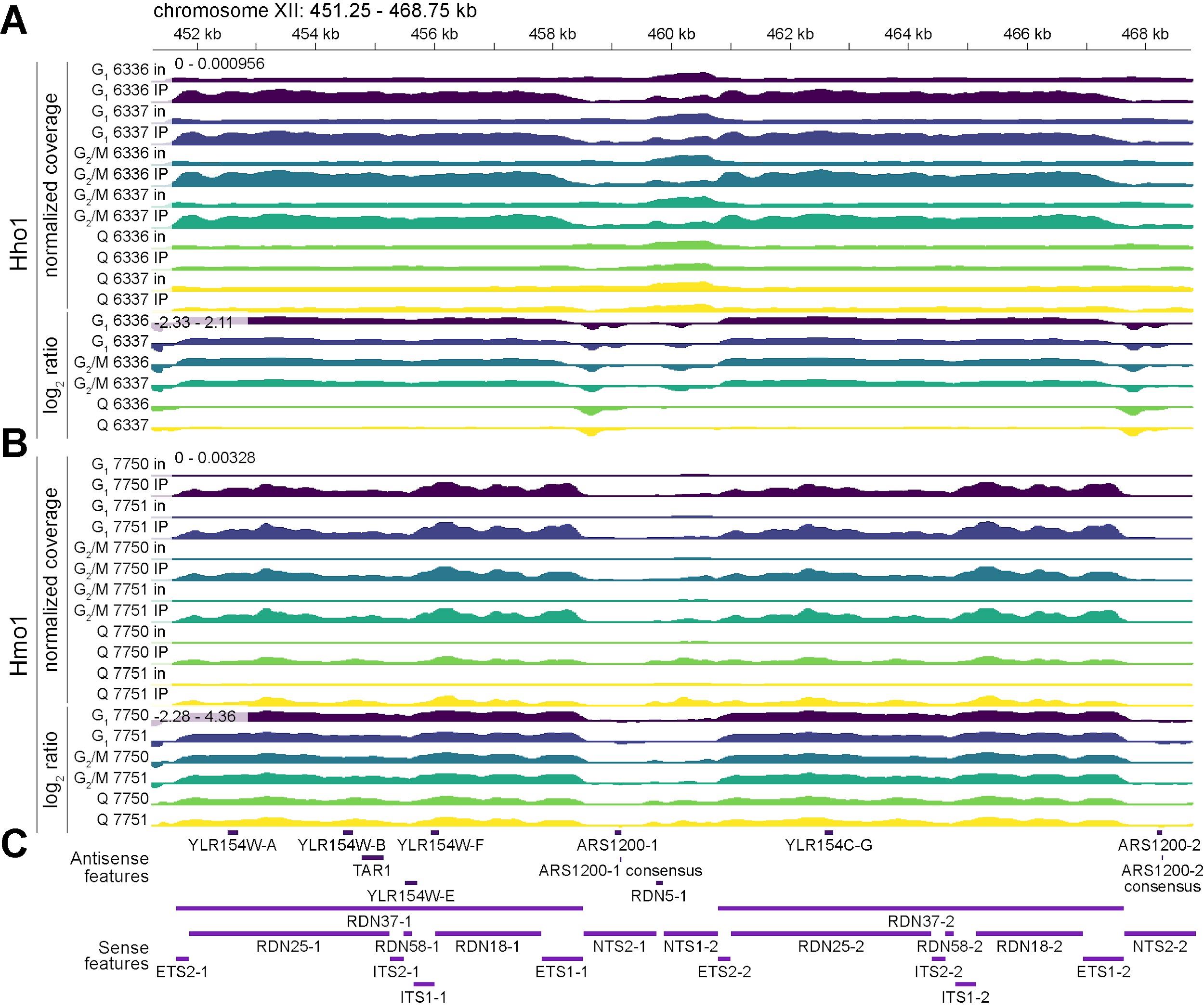
Figure 1. Normalized coverage and log2(IP/input) signal tracks at the S. cerevisiae rDNA locus. ChIP-seq signal tracks at the ribosomal DNA (rDNA) locus (chromosome XII, 451,250–468,750 bp) showing normalized coverage (top) and log2(IP/input) ratios of normalized coverage (bottom). Normalized coverage tracks represent fragment densities as probability distributions (see Data analysis F), while log2(IP/input) ratio (“log2 ratio”) tracks indicate relative enrichment (positive values) or depletion (negative values) of immunoprecipitated chromatin compared to input (see Data analysis G). Together, these metrics provide complementary views of DNA–protein interaction dynamics, allowing for relative comparisons across samples. Rows labeled “in” correspond to input normalized coverage; rows labeled “IP” correspond to immunoprecipitate normalized coverage. “G1” refers to cells in the G1 phase of the cell cycle, “G2/M” represents cells in the G2 and M phases, and “Q” indicates quiescent cells. Strains 6336/6337 and 7750/7751 are independent biological replicates. All tracks are binned at 30-bp resolution, with y-axis ranges shown above the initial normalized coverage and log2 ratio tracks; for log2 ratio tracks, the center line is set at 0. (A) Tracks for Hho1 (histone H1). (B) Tracks for Hmo1 (chromatin-associated high mobility group protein). (C) Annotated genome features from the GFF3 (see Data analysis A), separated by sense (maroon) and antisense (purple) strands.
G. Compute log2 ratios of IP to input normalized coverage
This section covers the computation of log2-transformed ratios of IP to input signal tracks, a standard method for evaluating ChIP-seq enrichment relative to background. The transformation is applied to corresponding IP and input normalized coverage tracks (see Data analysis F), producing log2 ratios that represent fold enrichment (Figure 1).
To compute per-sample log2(IP/input) normalized coverage ratios, run execute_compute_signal.sh. Refer to workflow.md for an example, including the generation of structured sample tables (see General note 34) that group corresponding IP and input files with values associated with script arguments. These include computed minimum input depth values (see General notes 35 and 36), which are passed as arguments to the --dep_min parameter of execute_compute_signal.sh to replace denominator (input) values below this threshold. This mitigates extreme ratio values and improves numerical stability.
H. Compute IP efficiency with siQ-ChIP
This section focuses on the computation of IP efficiency using the siQ-ChIP method [5,16]. At the core of siQ-ChIP is the concept that the immunoprecipitation of chromatin fragments represents an equilibrium binding reaction, in which reactants and products balance dynamically, governed by classical mass conservation laws, which state that total chromatin remains constant throughout the reaction. Mass conservation principles enable the experimentally measured IP mass to be interpreted as the result of a competitive binding reaction, influenced by antibody affinities and the concentrations of chromatin and antibodies. Sequencing reveals the genomic distribution of the IP product, recorded as normalized coverage (see Data analysis F).
The quantitative scale of siQ-ChIP, expressed in absolute physical units, is defined by the product of this sequencing-derived distribution and the IP mass, measured through methods such as fluorometric quantification (e.g., Qubit) or spectrometry (e.g., NanoDrop; see General notes 8, 37, and 38). Because these measurements are necessary to compute the siQ-ChIP scaling factor (α), the method requires quantifiable amounts of immunoprecipitated DNA (see General note 39). By establishing a quantitative scale, siQ-ChIP enables a precise measure of IP reaction efficiency, expressed as the ratio of bound (IP) signal to total (input) signal for any genomic interval. It is recommended to verify that an antibody yields consistent normalized coverage—i.e., stable signal—across different concentrations in ChIP-seq benchwork (see General note 40), as this supports the reliability of the efficiency measurement [5,7]. For additional discussion on how siQ-ChIP reinforces best practices intrinsic to ChIP-seq, see General notes 6 and 7.
To generate siQ-ChIP IP efficiency tracks, we compute a proportionality constant, α, that connects the sequencing-derived data to the underlying IP reaction dynamics. Specifically, α is a scaling factor—essentially the IP efficiency per Equation 6 of [16], derived from variables such as the total DNA mass in the IP product, etc. (see General notes 37 and 38)—ensuring the signal tracks reflect absolute, rather than relative, quantities (see General note 8). By multiplying α by the ratio of IP normalized coverage to input normalized coverage, siQ-ChIP generates a quantitative measure of protein–DNA binding efficiency, consistent with the physical scale of the IP reaction. This approach also extends to comparing different chromatin targets, provided that each antibody is validated for consistent performance under matched or saturating IP conditions (see General note 41).
In the following workflow, we determine α and use it to compute siQ-ChIP IP efficiency tracks from normalized coverage (see Data analysis F). Consult workflow.md for a detailed example of the following steps:
1. Define variables for serialized strings representing the corresponding IP and input BAM files (see Data analysis E). Specify a tab-separated metadata table containing the experimental parameters needed to compute α for each sample (Table 5; see Software and Datasets A; also, the metadata table used in this protocol is available for download from the project repository and GEO).
2. Pass these values to execute_calculate_scaling_factor.sh to compute sample-specific α values. This script processes the IP and input BAM files along with the metadata table of siQ-ChIP parameters to calculate proportionality constants. The table is programmatically parsed to match IP-input sample pairs with corresponding parameters (see Troubleshooting 5). File paths, computed α values, and related parameters are saved to a structured sample table for downstream parsing (see General note 34).
3. To generate siQ-ChIP-scaled signal tracks in bedGraph format, extract computed α values, corresponding IP and input BAM files, and minimum input depth values (see General notes 35 and 36) from the structured sample table. Convert BAM file paths to their associated normalized coverage bedGraph paths, then pass the extracted values, including scaling factors, to execute_compute_signal.sh. For each sample, the script scales the ratio of IP to input normalized coverage by multiplying it with α, generating IP efficiency tracks.
I. Compute spike-in-scaled signal
Here, we cover the computation of spike-in-scaled signal [15], a semiquantitative method that attempts to account for variability in ChIP-seq experiments by using exogenous chromatin as a reference to scale endogenous signal [11–15]. Initially, spike-in scaling was considered a practical alternative to standard sequencing depth normalization [11,15], which assumes relatively constant global signal levels across samples and is therefore inadequate for detecting biological changes that affect overall protein abundance, such as epitope masking by chromatin remodeling or chemical or genetic epitope depletion. Spike-in scaling can reveal global shifts in protein–DNA interaction levels, but it relies on several implicit and rarely validated assumptions (see General note 42). While the FLAG-tagged system used in this protocol mitigates some common issues (Tables 3 and 5; see General note 11), key limitations persist (see General note 42).
siQ-ChIP provides a more rigorous alternative, using the quantitative properties of the immunoprecipitation reaction to compute absolute protein–DNA interaction levels from experimental data (see General note 42). This approach eliminates the need for exogenous controls, addressing the limitations of spike-ins while enabling reliable comparisons across regions, samples, and conditions. Though steps for spike-in scaling are included here for contextual reference, we strongly recommend using siQ-ChIP and normalized coverage instead, as these methods provide more reliable and effective tools for, respectively, absolute and relative ChIP-seq analyses. Figure 2 shows representative tracks generated using both the spike-in and siQ-ChIP methods.
The following steps outline the computation of spike-in-scaled signal, with an example provided in workflow.md:
1. Define variables for serialized strings representing corresponding IP and input BAM files for both the main (S. cerevisiae) and spike-in (S. pombe) model organisms (see Data analysis E).
2. Run execute_calculate_scaling_factor.sh to calculate sample-specific spike-in scaling factors. This script processes the main and spike-in IP and input BAM files, recording computed scaling coefficients, file paths, minimum input depth values (see General notes 35 and 36), and related parameters in a structured sample table for use in downstream steps (see General note 34).
3. Optionally, use relativize_scaling_factors.py with the structured sample table to adjust each sample’s spike-in coefficient within a group to the maximum value in that group. This places the scaling factors on a relative scale from 0 to 1 (see General note 43).
4. Extract computed scaling factors along with corresponding S. cerevisiae IP and input BAM files from the structured sample table. Convert BAM file paths to their associated normalized coverage bedGraph paths, then pass the extracted values and coefficients—whether relativized in step I3 or not—to execute_compute_signal.sh. For each sample, the script calculates the IP-to-input coverage ratio and applies the scaling factor to generate the final spike-in-scaled signal tracks.
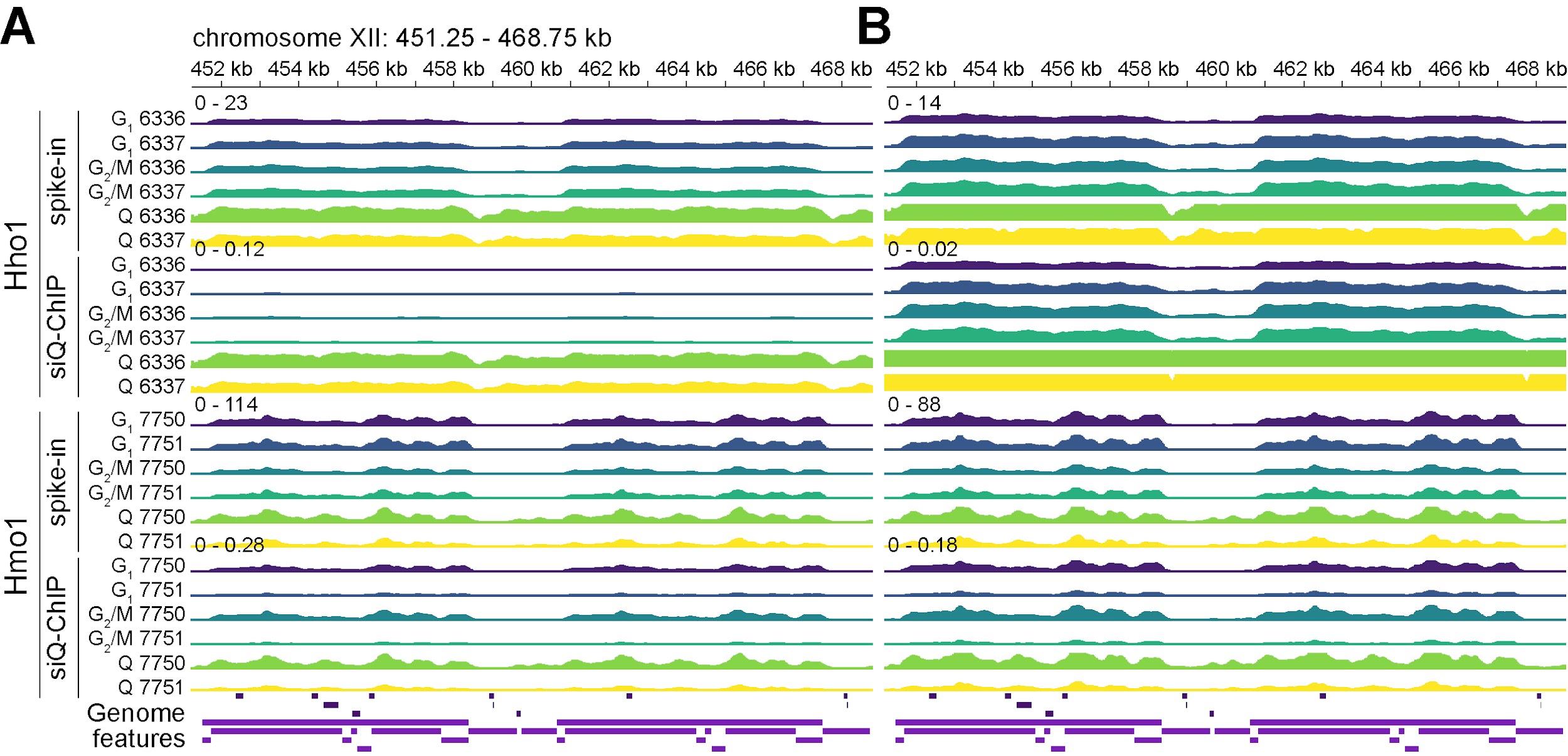
Figure 2. Spike-in-scaled signal and siQ-ChIP IP efficiency tracks at the S. cerevisiae rDNA locus. ChIP-seq signal tracks at the ribosomal DNA (rDNA) locus (chromosome XII, 451,250–468,750 bp) showing spike-in-scaled signal and siQ-ChIP IP efficiency for Hho1 (histone H1) and Hmo1 (chromatin-associated high mobility group protein). Genome features are displayed in the final row, separated by strand (maroon: antisense; purple: sense). All tracks are binned at 30 bp resolution, with y-axis ranges shown above the initial spike-in-scaled signal and siQ-ChIP IP efficiency tracks. “G1” refers to cells in the G1 phase of the cell cycle, “G2/M” represents cells in the G2 and M phases, and “Q” indicates quiescent cells. Strains 6336/6337 and 7750/7751 are independent biological replicates. (A) Hho1 (top) and Hmo1 (bottom) tracks, autoscaled separately for spike-in-scaled signal and siQ-ChIP IP efficiency, considering all conditions (G1, G2/M, and Q). (B) Hho1 (top) and Hmo1 (bottom) tracks, autoscaled separately for spike-in-scaled signal and siQ-ChIP IP efficiency, excluding Q tracks from the autoscaling. For a comparison of spike-in scaling and siQ-ChIP IP efficiency, including their sensitivity to variations in IP conditions, see General notes 42 and 44.
J. Visualize signal tracks with IGV
To visually explore signal tracks with respect to organism chromosomes and feature annotations, follow these steps:
1. Run IGV.
After installing IGV (see Procedure D), launch IGV by double-clicking its application icon.
2. Load a FASTA genome.
In IGV, go to Genomes > Load Genome from File… and select a FASTA file, such as the S. cerevisiae/S. pombe combined genome (see Data analysis A). If necessary, decompress the file first.
3. Load a corresponding GFF3 file.
Navigate to File > Load from File… and select a GFF3 file, such as the S. cerevisiae/S. pombe combined GFF3 file (see Data analysis A). Alternatively, drag and drop the file into IGV’s interface. The file can be compressed or not.
4. Load bedGraph signal tracks (see Data analysis F, G, H, and I).
Load signal tracks by repeating the same process as in step J3.
This configuration provides an interactive platform for examining signal tracks in the context of genomic features and annotations.
Validation of protocol
Parts of this protocol have been implemented and validated for consistency with data processing in the following research articles:
• Generation of siQ-ChIP IP efficiency [5]. Validation details are available in the Markdown notebook validate_siq_chip.md within the protocol repository.
• Normalized coverage and siQ-ChIP IP efficiency generation [16]. Validation details are available in the Markdown notebook validate_siq_chip.md within the protocol repository.
• Read and alignment processing [46].
General notes and troubleshooting
General notes
1. What are reads?
In NGS, reads refer to the DNA sequences generated by sequencing platforms. This protocol focuses on ChIP-seq datasets with reads generated on Illumina platforms.
Illumina uses a process called “sequencing by synthesis” [47], where DNA fragments from ChIP-seq libraries—collections of DNA fragments enriched for specific protein–DNA interactions—are attached to a flow cell and amplified to form clusters, each representing many copies of a single fragment. Sequencing occurs by synthesizing the complementary strand and incorporating fluorescently labeled nucleotides, one at a time. As each nucleotide is added, a camera captures the fluorescent signal, allowing the sequence to be determined. These sequences, often called “short reads,” typically range from 50 to 300 base pairs, depending on platform specifications.
Reads are typically stored in the FASTQ file format, which includes both sequence data and quality scores indicating the confidence level of each nucleotide base call. Analysts can use these scores to identify and filter out low-quality data. Depending on the platform, reads can be single-end, where sequencing occurs from one end of the fragment, or paired-end, where sequencing occurs from both ends (see General note 2).
2. Contrasting paired- and single-end short-read sequencing
Paired-end short-read sequencing involves sequencing both ends of DNA fragments, effectively demarcating entire fragments generated during processes such as ChIP-seq library preparation (see General note 4). This approach eliminates the need for fragment modeling as performed with single-end sequenced data—as detailed in publications such as [48,49]—enabling more accurate identification of protein-DNA binding sites (e.g., through peak calling) and improving the resolution of closely spaced binding events. Additionally, paired-end sequencing enhances alignment accuracy to repetitive or highly similar genomic regions, reducing ambiguity for reads that might otherwise align to multiple locations [50]. Despite these advantages, single-end sequencing, which sequences only one end of DNA fragments, was historically simpler and less expensive. However, advancements in sequencing technology and economies of scale from widespread adoption have led to reduced costs for paired-end sequencing.
3. What are reference genomes?
A reference genome is a digital database of nucleic acid sequences that represents the overall genome structure and typical set of feature annotations (e.g., genes and other genomic features) for a species. It serves as a standard for aligning reads (see General notes 1 and 2) from ChIP-seq and other genomic assays. Constructed by sequencing DNA from one or more individuals of a species, a reference genome is assembled into a contiguous sequence by piecing together read data from various sequencing technologies. For many species, it is a composite sequence that aims to capture the genetic diversity of the species rather than representing any single individual. Many reference genomes are continuously updated and refined as new data and technologies become available.
4. ChIP-seq signal represents the genome-wide fragment distribution
In ChIP-seq, sequenced reads originate from DNA molecules captured during immunoprecipitation (see General note 1). During library generation, the process of converting DNA into a form compatible with sequencing, the molecules are sheared, and adapters are ligated to the resulting fragments. Then, either single- or paired-end sequencing is performed (see General note 2). After sequencing, computational methods use aligned reads to infer the original fragment sizes and genomic locations (see Data analysis E). The resulting signal tracks—before normalization or any other adjustments—represent the distribution of inferred fragments across the genome, forming the basis for visualizing protein–DNA interactions.
5. What is data normalization?
In bioinformatics, normalization typically means making datasets comparable by adjusting for systematic biases or effects that are not of primary interest. For example, in ChIP-seq experiments, variations in cell state, sequencing depth, sample preparation, or library composition can introduce biases that affect the apparent enrichment of protein–DNA interactions. Normalization methods adjust for these discrepancies, aiming to enable more accurate comparisons within and across samples and experimental conditions.
6. Best practices in ChIP-seq and their roles in siQ-ChIP
siQ-ChIP emphasizes key technical practices in ChIP-seq that enhance reproducibility and improve data interpretation—practices that should be standard regardless of the normalization method used. These include the following:
a. Measuring and reporting input and IP DNA masses: Accurately quantifying input and IP DNA amounts is important for improving reproducibility and standardizing data reporting. This practice provides essential context for interpreting enrichment and should be routine in ChIP-seq experiments, regardless of the normalization method.
b. Characterizing antibody behavior using isotherms: Antibody binding strongly influences ChIP-seq signal but is often treated as a black box. siQ-ChIP uses isotherm-based measurements to assess antibody behavior (see General note 7), helping to differentiate between on- and off-target binding when information about target chromatin abundance is available (e.g., by mass spectroscopy). This approach increases confidence in specificity and provides deeper insights into immunoprecipitation efficiency.
c. Careful chromatin fragmentation: Fragmentation directly impacts ChIP-seq results, affecting both resolution and sensitivity in detecting protein–DNA interactions. siQ-ChIP encourages researchers to optimize fragmentation conditions based on the biological question at hand. This level of attention should be standard practice across all ChIP-seq experiments.
Beyond these technical considerations, siQ-ChIP offers a major advantage by providing empirical measures that help explain sources of variability between experiments. When results fail to replicate, siQ-ChIP enables researchers to investigate potential causes by examining antibody isotherms, fragment size distributions, and immunoprecipitation conditions. Many ChIP-seq studies fail—partially or entirely—to integrate these physical factors with sequencing data, creating gaps that limit reproducibility, hinder data interpretation, and likely reduce the biological insights that can be gained from ChIP-seq experiments.
7. Understanding antibody binding isotherms in ChIP-seq
An isotherm is an empirical relationship that describes how one variable (e.g., binding, adsorption, or phase change) depends on another (e.g., concentration or pressure) while temperature remains constant. Isotherms are widely used in chemistry, biochemistry, and physics to characterize binding, adsorption, and phase transitions.
In this protocol, isotherms refer to binding curves that describe how an antibody interacts with its target under equilibrium conditions, which are influenced by antibody concentration, target abundance, and binding affinity. These binding curves plot the fraction of target molecules bound at different antibody concentrations, helping to quantify binding affinity and specificity.
Isotherms provide insights into binding strength, which directly influences ChIP-seq enrichment. Notably, antibody binding to chromatin is not governed by a single binding constant, as different antibodies exhibit a range of interaction strengths across chromatin contexts. For examples of such variability, including documented cases of antibodies recognizing multiple histone modifications with different affinities, see [51] and the associated Histone Antibody Specificity Database (histoneantibodies.com).
Given this variability, analyzing isotherms allows researchers to assess whether an antibody binds primarily to its intended target (on-target) or also interacts with unintended sequences (off-target). If the amount of immunoprecipitated chromatin exceeds what is expected based on target abundance, the antibody may be binding through additional, unintended epitopes [7]. Conversely, if little chromatin is recovered regardless of conditions, the antibody may have poor enrichment efficiency [7]—though this should be interpreted with caution for rare targets, where low recovery may still reflect specific binding (see General note 39). Because binding strength directly affects ChIP-seq enrichment, identifying the concentration at which an antibody reaches saturation (i.e., when increasing its concentration no longer increases recovery) helps optimize immunoprecipitation efficiency.
siQ-ChIP incorporates isotherm-based measurements to empirically evaluate antibody performance, rather than assuming all antibodies function equally well. This approach improves normalization and reproducibility in ChIP-seq experiments. For example, on a practical level, having an established isotherm for one antibody lot allows researchers to compare it with a new lot, helping to re-establish confidence in reagent consistency.
8. Distinguishing quantitative, semiquantitative, absolute, and relative scales for signal.
The terms quantitative, semiquantitative, absolute, and relative describe different degrees of measurement precision and interpretability in data analyses (Table 6).
• Quantitative methods provide numerically precise, reproducible values on a defined scale, often expressed in absolute units (e.g., molarity, nanograms, etc.).
• Absolute measurements, a subset of quantitative methods, use fixed, standardized units or ratios, enabling direct comparisons across datasets.
• Semiquantitative methods fall between qualitative (i.e., descriptive or categorical) and quantitative approaches, generating numerical values that allow for comparative analysis under certain assumptions but lack an absolute scale or precise standardization.
• Relative measurements describe values in proportion to each other, conveying enrichment or fold-change without defining an exact unit.
Table 6. Comparisons of data scales. Summary of the characteristics of quantitative, absolute, semiquantitative, and relative scales, highlighting their advantages, limitations, and interrelationships.
| Scale | Advantages | Limitations | Interrelationships |
|---|---|---|---|
| Quantitative | Precise, reproducible values; allows for direct comparisons across datasets | Requires controlled conditions and calibration; sensitive to technical variation | Includes absolute measurements as a subset; re-scalable for relative comparisons |
| Absolute | Direct measurement; enables cross-experiment comparisons | Can be difficult to achieve in practice due to standardization requirements | Subset of quantitative measurements, but distinct in that it defines signal in physical units or ratios |
| Semiquantitative | Allows for approximate comparisons when absolute values are unavailable | Lacks absolute scale, making results dependent on context and sometimes less reproducible | Overlaps with relative measurements but applies additional assumptions for comparative interpretation |
| Relative | Enables internal comparisons within an experiment; does not require external standards | Cannot determine absolute amounts; can be misleading if normalization assumptions are violated | Often used in semiquantitative methods; can also be applied to quantitative data |
Normalized coverage is a relative measure of fragment density, represented as a probability distribution (see Data analysis F and General note 33); this ensures comparability within and across datasets but does not provide absolute quantification (Figure 1). Similarly, log2(IP/input) ratios provide a relative measure of enrichment but do not account for differences in IP efficiency and others (see Data analysis G; Figure 1). In contrast, siQ-ChIP IP efficiency is quantitative, as it directly measures the proportion of target chromatin recovered in an IP relative to total chromatin input, basing signal in absolute physical units (see Data analysis H and General notes 37 and 38; Table 5; Figure 2). Finally, spike-in normalization is semiquantitative, rescaling data proportionally with an external reference without establishing absolute quantities (see Data analysis I and General note 42; Figure 2). While semiquantitative measurements are often relative, not all relative comparisons are semiquantitative, as relative scaling can be applied to quantitative data too.
9. Foundational bioinformatics resources for beginners
For researchers new to computational analysis, gaining familiarity with basic bioinformatics skills will help in using this protocol. Below are some recommended free resources covering fundamental topics such as working with the command line, version control with Git, and general bioinformatics concepts.
Command-line and shell scripting basics: These resources introduce the Bash command-line interface as a bioinformatics tool. They cover important skills such as directory navigation, file management, text processing, variable usage, wildcards, input/output redirection, and scripting automation with loops, among other fundamental concepts.
• Introduction to the Command Line for Genomics – Data Carpentry [52]
• Shell for Bioinformatics – Harvard Chan Bioinformatics Core (HCBC) [53]
• Unix 1 – Cold Spring Harbor Laboratory (CSHL) Programming for Biology (PB)
• Unix Shell – Software Carpentry [54]
Working with Git and version control: These resources introduce Git as a tool for managing code, tracking changes, and enabling collaboration in bioinformatics. Topics include initializing and cloning repositories, staging and committing changes, branching and merging, navigating commit history, and working with remote repositories such as GitHub.
• Pro Git – A free online book [55]; recommended chapters: Getting Started and Git Basics.
• Version Control with Git – Software Carpentry [56]
• See also General notes 17 and 18 and Troubleshooting 4.
Fundamentals of bioinformatics: The following resources introduce key bioinformatics concepts and practices, including computational methods for analyzing biological data, programming for data processing, and strategies for organizing and interpreting sequencing data. Topics include ChIP-seq analysis—reinforcing, expanding, or complementing concepts in this protocol—scripting in Python and R, and interactive exercises covering various aspects of bioinformatics.
• Introduction to ChIP-seq – HCBC
• Introduction to Python – CSHL PB
• Introduction to R – HCBC [57]
• Investigating chromatin biology using ChIP-seq and CUT&RUN – HCBC [58]
• Rosalind
10. ChIP-seq data processing and signal computation in the context of ribosomal DNA
This protocol includes specific considerations for processing ChIP-seq data and interpreting signals at the ribosomal DNA (rDNA) locus in S. cerevisiae. Our focus on rDNA reflects its regulatory significance and its role in cellular transitions, particularly between quiescence—a reversible state of cell cycle withdrawal—and active proliferation. More broadly, rDNA biology intersects multiple areas of research, including chromatin regulation, nuclear organization, and translation, making it relevant to many research groups. Since existing ChIP-seq protocols rarely address data processing and signal interpretation at rDNA, we explicitly include these aspects. While analyzing ChIP-seq data at rDNA is not complex, it requires data processing steps that are not commonly discussed in other protocols. These steps, discussed in Data analysis E and General note 30, account for factors specific to repetitive sequences in reference genomes, a category that includes rDNA. However, these data processing steps are broadly applicable to ChIP-seq analysis across the genome—not just at rDNA—and to other model organisms beyond S. cerevisiae.
11. Overview of ChIP-seq sample preparation
S. cerevisiae cells were arrested at distinct cell cycle stages prior to chromatin immunoprecipitation. Cells arrested in the first gap phase of the cell cycle (G1) were obtained by growing cultures to an optical density at 660 nm (OD660) of 0.2 and treating them with 5 μg/mL alpha factor for 80 min. Cells arrested in the second gap phase of the cell cycle (G2) and mitosis (M), collectively termed G2/M cells, were grown to an OD660 of 0.7 and treated with 15 μg/mL nocodazole for 120 min. Cells in quiescence (Q), a reversible state of cell cycle withdrawal, were generated by culturing for 7 days and purified via Percoll density gradient centrifugation [59,60]. Cell cycle arrest and quiescence entry were confirmed by microscopy and flow cytometry.
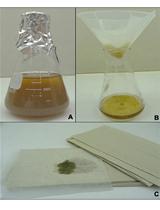
Cells were crosslinked with 1% formaldehyde for 20 min, quenched with 125 mM glycine, washed with Tris-buffered saline, and lysed by bead beating. Chromatin was fragmented by two rounds of sonication using a Bioruptor UCD-200 set to high power for 15 min, with 30 s on/off cycles. For chromatin immunoprecipitation, 1 μg of S. cerevisiae chromatin was combined with 2.65 ng of S. pombe spike-in chromatin in a total of 300 μL sonication buffer. A 20 μL aliquot was set aside as input; the remaining 280 μL was used for immunoprecipitation.
Chromatin was incubated with 2 μL of FLAG M2 antibody (Sigma, F1804) and 20 μL of Dynabeads Protein G (Invitrogen). Antibody conjugation was performed by incubating beads in phosphate-buffered saline with 0.1% Tween-20 (PBS-T) for 60 min at room temperature, followed by one PBS-T wash and one FA buffer wash. Beads were then incubated with chromatin for 90 min. Following immunoprecipitation, beads were sequentially washed with FA buffer (3×), high-salt FA (FA-HS) buffer (2×), and radioimmunoprecipitation assay (RIPA) buffer (1×). Chromatin was eluted at 75 °C, and eluates were pooled for a final volume of 40 μL.
Crosslinks were reversed overnight at 65 °C, followed by sequential digestion with 10 mg/mL RNase A (55 °C, 1 h) and 10 mg/mL Proteinase K (55 °C, 3 h). DNA was purified using a MinElute PCR Purification Kit (Qiagen) and quantified using a Qubit 4 Fluorometer (Invitrogen), which measures DNA concentration via fluorescence-based detection.
Due to the practical constraints of processing multiple samples simultaneously, input and IP chromatin were prepared in three separate batches (Table 7), maintaining equivalent chromatin and bead amounts.
ChIP-seq libraries were prepared using the Ovation Ultralow System V2 (Tecan). Libraries were generated from 2 ng of DNA, amplified via 11 cycles of PCR on an S1000 Thermal Cycler (Bio-Rad), and purified using AMPure XP beads (Agencourt) to retain fragments greater than 100 bp in size. Library quality was assessed using a TapeStation system. Samples were pooled to 2 nM each and sequenced on a NextSeq 2000 (Illumina) with 50 bp paired-end reads and single 8 bp indexes.
Table 7. Chromatin input and immunoprecipitation sample details and DNA concentrations. Summary of chromatin samples used for ChIP-seq, including input and immunoprecipitated (IP) DNA (“type”) for Hho1 and Hmo1 (“factor”) across different strains (“strain”) and cell cycle stages (“stage”). Metadata includes batch numbers (“batch”), experimental and library preparation dates (“date_exp” and “date_library”), and DNA concentrations (ng/μL) measured post-purification (“conc_dna”).
| Type | Factor | Strain | Stage | Batch | date_exp | date_library | conc_dna |
|---|---|---|---|---|---|---|---|
| input | Hho1 | yTT6336 | G1 | 2 | 2023-0825 | 2023-0831 | 6.04 |
| input | Hho1 | yTT6337 | G1 | 1 | 2023-0718 | 2023-0831 | 6.76 |
| input | Hho1 | yTT6336 | G2/M | 2 | 2023-0825 | 2023-0831 | 8.74 |
| input | Hho1 | yTT6337 | G2/M | 1 | 2023-0718 | 2023-0831 | 7.1 |
| input | Hho1 | yTT6336 | Q | 2 | 2023-0825 | 2023-0831 | 6.06 |
| input | Hho1 | yTT6337 | Q | 1 | 2023-0718 | 2023-0831 | 5.8 |
| input | Hmo1 | yTT7750 | G1 | 1 | 2023-0718 | 2023-0831 | 6.66 |
| input | Hmo1 | yTT7751 | G1 | 3 | 2023-0831 | 2023-0831 | 5.3 |
| input | Hmo1 | yTT7750 | G2/M | 1 | 2023-0718 | 2023-0831 | 2.7 |
| input | Hmo1 | yTT7751 | G2/M | 3 | 2023-0831 | 2023-0831 | 7.78 |
| input | Hmo1 | yTT7750 | Q | 1 | 2023-0718 | 2023-0831 | 5.66 |
| input | Hmo1 | yTT7751 | Q | 3 | 2023-0831 | 2023-0831 | 8.88 |
| IP | Hho1 | yTT6336 | G1 | 2 | 2023-0825 | 2023-0831 | 0.224 |
| IP | Hho1 | yTT6337 | G1 | 1 | 2023-0718 | 2023-0831 | 0.42 |
| IP | Hho1 | yTT6336 | G2/M | 2 | 2023-0825 | 2023-0831 | 0.55 |
| IP | Hho1 | yTT6337 | G2/M | 1 | 2023-0718 | 2023-0831 | 0.51 |
| IP | Hho1 | yTT6336 | Q | 2 | 2023-0825 | 2023-0831 | 9.74 |
| IP | Hho1 | yTT6337 | Q | 1 | 2023-0718 | 2023-0831 | 5.88 |
| IP | Hmo1 | yTT7750 | G1 | 1 | 2023-0718 | 2023-0831 | 0.704 |
| IP | Hmo1 | yTT7751 | G1 | 3 | 2023-0831 | 2023-0831 | 0.268 |
| IP | Hmo1 | yTT7750 | G2/M | 1 | 2023-0718 | 2023-0831 | 0.454 |
| IP | Hmo1 | yTT7751 | G2/M | 3 | 2023-0831 | 2023-0831 | 0.282 |
| IP | Hmo1 | yTT7750 | Q | 1 | 2023-0718 | 2023-0831 | 2.28 |
| IP | Hmo1 | yTT7751 | Q | 3 | 2023-0831 | 2023-0831 | 1.23 |
12. On find_files.sh
The utility script find_files.sh is designed to simplify the process of locating files in a specified directory using the find command (see, for example, man7.org/linux/man-pages/man1/find.1.html and ss64.com/mac/find.html). The script minimizes the need for manual file listing, supports complex filtering options, and promotes reproducibility in bioinformatics workflows. It supports searches for various file types, including FASTQ, BAM, and TXT files, returning results as a single comma-separated string (or, when called with flag --fastqs for FASTQ files, a single semicolon- and comma-separated string) that can be passed to driver scripts. For more information, see the find_files.sh documentation.
13. What are shells?
A shell is a command-line interpreter that allows users to interact with the operating system by executing commands and running scripts, among many other things. Common shells include Bash (Bourne Again Shell), Zsh (Z shell), and Fish (Friendly Interactive Shell), each with distinct features and syntax. This protocol is designed to work with Bash.
14. The role of environments in software management
Isolating software installations in environments prevents conflicts between different versions of packages (bundled collections of software) or libraries (prewritten code modules that programs use to perform specific tasks). For example, consider a scenario where two projects require different versions of the programming language Python. In this context, these versions are called “dependencies” because each project depends on a specific version to function correctly: one might require an older version of Python for a key program, while the other needs a newer version to access features available only in recent releases. Without environments, installing packages globally can create conflicts: updating software for one project may inadvertently break dependencies required by another. Environments solve this issue by keeping software installations separate, ensuring that changes in one environment do not interfere with others or affect system-level applications. This isolation minimizes errors and maintains system stability.
15. On terminals and terminal sessions
A terminal is an interface for interacting with the operating system via text commands, allowing users to execute commands, navigate directories, manipulate files, and run programs—among many other things—without relying on a graphical user interface. Many bioinformatics workflows, including this protocol, rely on using a terminal. When a terminal is opened, it starts a terminal session, which runs a command-line shell (see General note 13), which processes commands and manages the session environment (see General note 14).
16. On the HOME directory
On Linux and macOS, the HOME directory is the default location for storing personal files, configurations, and software settings, among other things. Each user on a system has a unique HOME directory, typically as follows:
• Linux: /home/username
• macOS: /Users/username
The HOME directory is referenced by the environment variable ${HOME}, allowing users quick navigation with
# Navigate to HOME explicitly
cd "${HOME}"
# Navigate to HOME using its shortcut, the tilde (~)
cd ~
Many applications store user-specific settings and cached files in hidden files—those whose names begin with a period—and subdirectories within the HOME directory (e.g., ~/.bashrc, ~/.config, ~/.ssh). When working with bioinformatics tools and package managers such as Miniforge, the HOME directory is a typical default location for installations and environment configurations.
17. Understanding version control, repositories, and Git
Version control is a system for tracking file changes in a repository, a structured directory that organizes and manages project files over time. It enables users to manage revisions, collaborate, and return to previous file versions or states as needed. Git, a widely used version control system, synchronizes a local copy of a repository—the version stored on an individual system—with a remote repository, such as one on GitHub (github.com), which serves as the central source for updates and collaboration.
18. What are commits, pushes, and branches in Git?
In Git, committing changes (e.g., git commit or git commit -m “Description of changes”) saves modifications to a repository’s history, creating a checkpoint that tracks progress, preserves previous file versions, and allows changes to be undone if needed. However, commits only affect the local repository and do not automatically update the remote repository.
To update the remote repository, committed changes must be explicitly pushed:
git push
For example, a full workflow for committing and pushing changes might look like this:
# (Performed after editing documentation in script 'compute_signal.py')
git add ~/repos/protocol_chipseq_signal_norm/scripts/compute_signal.py
git commit -m "Edited documentation in 'compute_signal.py'"
git push origin main
In this command, “origin” refers to the remote repository where the changes will be pushed, and “main” refers to the “branch” being updated.
In Git, a branch is an independent version of a repository that allows changes to be made without affecting other branches. This enables multiple versions of a project to exist simultaneously. For example, many repositories have a “devel” for code development and testing before merging changes into the “main” branch, which typically contains the stable version of the code.
By default, “origin” refers to the primary remote repository when first cloned, and “main” is the default branch in many modern Git repositories (older repositories may use “master” instead). The command git push origin main updates the remote repository’s “main” branch with the committed changes.
This separation allows for local version control without immediately modifying shared project files in the remote repository. It also enables users to review and organize their changes before making them publicly available.
19. What does it mean for a program to be pre-compiled?
A pre-compiled program has already been translated from source code into machine-readable code, allowing it to run without further compilation. These programs are typically distributed as binaries—i.e., ready-to-run files that do not require building from source. Downloading a Julia binary, for example, provides an executable version of the language without the need for compilation.
20. What is a tarball?
A tarball is a kind of file that bundles multiple files and directories using the Tar (Tape Archive) program. Tarballs are often compressed to reduce file size, with formats like .tar, .gz, or .tgz (compressed with gzip), or .tar.xz (compressed with xz). Unpacking a tarball restores its contents back to their original state:
tar -xzf file.tar.gz # For gzip-compressed tarballs
tar -xJf file.tar.xz # For xz-compressed tarballs
Here, -x extracts the files, -z or -J handles decompression, and -f specifies the filename.
21. On the PATH variable
The PATH variable is an environment variable (${PATH}) that tells the shell (e.g., Bash, Zsh, etc.) where to look for executable programs. When a command is entered in the terminal, the shell searches the directories listed in PATH to find and run the program. By default, PATH includes system directories such as /usr/bin and /bin, but users can modify it to include additional locations. Appending new directories to PATH—as is done for Julia and Atria in this protocol—allows programs in those directories to be executed from any location without the need to specify full paths.
22. On shell configuration files
Shell (see General note 13) configuration files are scripts that run automatically when a terminal session starts (see General note 15), setting up the command-line environment (see General note 14) by defining system paths, aliases, environment variables, and other settings. The specific configuration file used depends on the shell type and whether the session is interactive (a user-initiated terminal session) or a login session (a session started upon logging in).
Common shell configuration files include:
• Bash (default on many Linux systems and older macOS versions)
~/.bashrc (for interactive non-login shells)
~/.bash_profile (for login shells)
• Zsh (default on modern macOS versions)
~/.zshrc (for interactive non-login shells)
~/.zprofile (for login shells)
To determine the current shell, run
echo "${SHELL}"
To determine the shell currently running in an active terminal session, use
echo $0
For most users, adding environment variables like PATH (see General note 21) to ~/.bashrc (Bash) or ~/.zshrc (Zsh) is appropriate.
23. On the term FASTA
FASTA is a plain-text format primarily used for storing nucleotide and protein sequences, though it can accommodate other symbolic sequence data. Its name comes from a sequence alignment program of the same name [61,62], which introduced an alignment algorithm and formalized the file format. The term FASTA derives from the phrase “FAST-All,” referring to the program’s speed in aligning nucleotide and protein sequences, among others. Due to its simplicity and broad applicability, the corresponding format became a bioinformatics standard. A FASTA file consists of one or more sequences, each preceded by a single-line definition (i.e., a header line) beginning with >. This line typically includes an identifier, followed by an optional description. The sequences themselves are written in standard IUPAC (International Union of Pure and Applied Chemistry) nucleotide or protein codes and can span multiple lines. For more details, see the following resources:
• A description of the FASTA format on the laboratory website of Yang Zhang at the University of Michigan (link; archived version).
• Tables of IUPAC nucleotide and protein (amino acid) codes on bioinformatics.org (link; archived version).
24. What is GFF3 and why is it used?
GFF3 (General Feature Format version 3) is a structured file format for annotated genome features. It defines elements such as genes, exons, and regulatory regions in a tab-delimited format, with each line representing a feature. A GFF3 file consists of nine fields, including sequence ID, source, feature type, start and end coordinates, score, strand, and metadata, which are stored in column 9 as key-value attribute pairs. GFF3 improves upon earlier versions (GFF1 and GFF2) with additional format standardization and support for extensive feature relationships. For example, it allows multi-level nesting, where genes can contain multiple transcripts, which in turn reference exons and other sub-features. Due to this structured format, GFF3 is widely used in genome browsers, comparative genomics analyses, and other bioinformatics applications.
25. On the conversion of URL-encoded characters and HTML entities in the S. cerevisiae GFF3 file
The raw S. cerevisiae GFF3 file contains URL-encoded characters (e.g., %20 for spaces) and HTML entities (e.g., β for β) in its attribute fields (column 9). While these encodings facilitate web-based data storage and representation, they can reduce readability and, in some cases, interfere with proper GFF3 file loading in genome browsers such as IGV.
To improve legibility and ensure compatibility with IGV, the following substitutions are applied during GFF3 processing:
• %20 to “ ” (space)
• %2C to “,” (comma)
• %3B to “,” (comma instead of semicolon, as GFF3 key-value attributes in column 9 are semicolon-delimited; converting %3B to semicolons disrupts attribute formatting in IGV)
• %28 to “(”
• %29 to “)”
• β (β) to “beta”
• ′ (') to “ prime”
• % (literal) to “ percent”
26. What are File Transfer Protocol (FTP) links?
FTP links are used to transfer files over the internet, typically between a user and a remote server. A standard protocol for downloading and uploading data, FTP is often used in bioinformatics to retrieve large sequencing datasets from public repositories. Unlike HTTP or HTTPS, which are built for web browsing, FTP is designed specifically for file transfers and is often accessed via command-line tools such as curl or wget or through FTP client software (e.g., FileZilla).
27. On the “assay_genotype_state_treatment_factor_strain/replicate” naming scheme
For legibility and reproducibility, we recommend user-defined filenames following the format “assay_genotype_state_treatment_factor_strain/replicate”. This structure places stable attributes (e.g., assay type) on the left and more variable attributes (e.g., replicates) on the right. Below is a breakdown of each attribute:
• “Assay” refers to the next-generation sequencing method used for the samples (e.g., RNA-seq, ATAC-seq, or Hi-C). However, rather than using the term ChIP-seq, we use “IP” (for immunoprecipitate) and “in” (for input) to distinguish between these two types of ChIP-seq data.
• “Genotype” refers to samples’ genetic background, e.g., WT (wild type) or SMC4-off (conditional depletion of SMC4 through a Tet-Off system).
• The term “state” signifies samples’ positions in the cell cycle. For example, samples could be in “log” (logarithmic) growth, a mixture of active cell cycle stages, or in specific stages of the cell cycle such as “G1” (G1), “G2M” (G2/M, i.e., a mixture of the G2 and mitotic stages), or “Q” (quiescence).
• “Treatment” signifies an experimental intervention applied to samples, such as a drug or control chemical. For example, H3K27me3 IP samples might be treated with a “vehicle” (control) or an EZH2 inhibitor.
• “Factor” represents the protein targeted for immunoprecipitation.
• If one or more attributes (such as state, genotype, or treatment) are not relevant for a particular set of samples, we omit them from the custom names.
Below is an example of how a custom name might be constructed, with the “state” and “treatment” attributes omitted as they are not relevant in this context. Also, FTP addresses (see General note 26) are replaced with ellipses for brevity.
Given the following row in the downloaded table:
run_accession sample_title fastq_ftp
SRR7175368 Brn1 in Log Replicate 1 Input...
Create the following custom name:
run_accession sample_title fastq_ftp custom_name
SRR7175368 Brn1 in Log Replicate 1 Input ... in_WT_log_Brn1_rep1
28. Best practices for downloading and naming files
To avoid confusion or errors in downstream analyses, we recommend against renaming downloaded files directly. Instead, retain the original filenames and create symbolic links (“symlinks”) with custom names. Symlinks, created using the ln -s command, act as pointers to the original files, allowing more intuitive, convenient naming without modifying the original files. This preserves file integrity while providing flexibility. For example, to create a symlink easy_interpretable_name.fastq.gz pointing to a raw sequencing file, do the following:
ln -s \
"${HOME}/path/to/fastqs/raw/complicated_original_name.fastq.gz" \
"${HOME}/path/to/fastqs/sym/easy_interpretable_name.fastq.gz"
We also advocate for managing downloads and symbolic link creation through TSV (or similar) files (see Data analysis C). This documents filenames and sources, reducing uncertainty and aiding troubleshooting.
29. Default adapter handling by Atria
If the arguments --adapter1 and --adapter2 (for paired-end sequenced reads) are not specified, Atria defaults to using Illumina TruSeq single and combinatorial dual index adapter sequences, which are suitable for most ChIP-seq applications:
• Adapter sequence 1: AGATCGGAAGAGCACACGTCTGAACTCCAGTCA
• Adapter sequence 2: AGATCGGAAGAGCGTCGTGTAGGGAAAGAGTGT
For more information, refer to the Atria and Illumina Adapter Sequences documentation.
30. On the determination of multi-mapping alignments by Bowtie 2.
The classification of multi-mapping alignments by Bowtie 2 involves complex criteria that extend beyond the scope of this protocol. For readers seeking a deeper understanding, the following resources provide detailed explanations:
• Bowtie 2 publications [28–30].
• Bowtie 2 manual.
• A detailed explanation in a blog post by John Urban (archived version), which offers a nuanced discussion on how Bowtie 2 defines and handles multi-mapping alignments (referred to as “true multireads” in the post).
31. What does it mean for alignments to be properly paired?
The definition of properly paired alignments varies by aligner. With Bowtie 2, the term “properly paired” refers to paired-end alignments where both reads align in a manner consistent with the expected orientation, distance, and fragment length determined during library preparation (see General notes 2 and 4). Typically, this means that the forward read and its corresponding reverse read align to the same chromosome (or reference sequence) in an inward-facing orientation and within a specified distance from each other. This distance is defined by the Bowtie 2 parameters --minins (minimum fragment length) and --maxins (maximum fragment length). In this protocol, we retain the default values for these parameters when running Bowtie 2. For more details, refer to the Bowtie 2 manual.
32. What are MAPQ scores?
Bowtie 2 assigns a mapping quality (MAPQ) score to each alignment, reflecting the confidence that the reported position is correct. The calculation of MAPQ scores varies across alignment programs, and Bowtie 2 uses a method that differs from the standard definition established in [63]; for more on that standard, refer to the Sequence Alignment/Map (SAM)Format Specification. A detailed explanation of Bowtie 2’s MAPQ calculation is beyond the scope of this protocol; however, for readers seeking a deeper understanding, the following resources provide in-depth information:
• Bowtie 2 publications [28–30].
• Bowtie 2 manual.
• Two in-depth blog posts by John Urban (linked here and here; archived versions here and here), which explain Bowtie 2’s MAPQ scoring in detail, including underlying concepts and code examples.
• A forum post by Devon Ryan on seqanswers.com [64] describing Bowtie 2’s MAPQ scoring logic by walking through a relevant C function.
Notably, when the MAPQ score assigned by Bowtie 2 exceeds 1, multi-mapping alignments are excluded from the data. This effectively prevents the analysis of signals at repetitive loci such as the S. cerevisiae rDNA locus. In this protocol, we filter for MAPQ ≥ 1 to exclude lower-quality multi-mapping alignments, particularly those with more than five mismatches to the reference genome (for more on this, see the blog posts by John Urban).
33. Distinguishing normalized coverage from sequencing coverage
Normalized coverage differs from—but is related to—sequencing coverage (often shortened to “coverage”), which describes how often bases in a reference genome (see General note 3) are covered by read alignments (i.e., the number of “mapped” bases; see General note 1) [65]. For example, if an NGS library is sequenced to 30× coverage, it means that, on average, each base in the reference genome is covered by 30 read alignments. Whereas coverage is computed from read alignments, normalized coverage is derived from read alignment-inferred fragments, which represent the original DNA molecules in ChIP-seq library preparations prior to fragmentation (see General note 4). These inferred fragments are then used to compute normalized coverage. In brief, coverage sums to mapped bases and measures “read depth”; normalized coverage sums to 1 and measures fragment density.
34. Sample table construction for signal track generation
Structured sample tables are generated to associate each IP sample with its corresponding input sample before computing log2-transformed ratios of normalized coverage, siQ-ChIP IP efficiency tracks, and/or spike-in-scaled signal tracks. These tables include necessary argument values (e.g., IP and input fragment depths), computed scaling factors (e.g., siQ-ChIP α proportionality constants or spike-in scaling factors), and minimum input depth values (see General note 35). Organizing this information in structured tables facilitates efficient parsing and ensures that related argument values remain linked, supporting reproducibility. Details on computing many of these argument values are provided in later sections; this preparatory step standardizes the workflow and streamlines data processing. Refer to workflow.md for more details.
35. Understanding minimum input depth values
When computing IP/input normalized coverage ratios, very small input values can produce extreme ratios. To prevent this, a minimum input depth value is used. If the input value is below this threshold, it is replaced by the minimum. This adjustment maintains numerical stability while preserving meaningful fold-change comparisons. The minimum input depth value for normalized coverage is calculated as the ratio of bin size—the genomic window used for signal computations—to the difference between effective genome size, which represents the alignable portion of the genome (see General note 36), and bin size: bin size ÷ (effective genome size – bin size).
36. On effective genome size
The effective genome size—i.e., the alignable fraction of the genome—is typically defined in one of two ways:
a. Counting the number of non-N bases in the reference genome. This approach is used when MAPQ filtering is not applied and/or when multi-mapping alignments are retained after MAPQ filtering.
b. Estimating the genome-wide count of unique “k-mers”—nucleotide substrings of length “k”, typically corresponding to the length of sequenced reads—as an approximation of the number of uniquely alignable bases in the genome. This approach is used when MAPQ filtering is applied and/or when multi-mapping alignments are excluded.
As alignments are filtered for MAPQ ≥ 1 in data processing, multi-mapping alignments with up to five mismatches are retained in the data (see Data analysis E and General note 30). Therefore, this workflow uses the first definition. Non-N bases are tallied with faCount, a utility in the UCSC Genome Browser suite [66]:
# Define variables
dir_bas="${HOME}/repos"
dir_rep="${dir_bas}/protocol_chipseq_signal_norm"
dir_fas="${dir_rep}/data/genomes/cerevisiae/fasta/proc"
fil_fas="${dir_fas}/S288C_R64-5-1_proc.fasta.gz"
# Check that faCount is available
if ! command -v faCount &> /dev/null; then
echo \
"Error: 'faCount' not found in PATH. The program can be" \
"installed with Conda/Mamba: 'bioconda::ucsc-facount'." >&2
fi
# Count number of non-N bases in genome
faCount -summary "${fil_fas}"
For comparison, here is an example of estimating the genome-wide count of unique k-mers. Since the read length is 50 bp, k-mer estimation is performed for 50-mers using unique-kmers.py, a script from the khmer software suite that applies HyperLogLog cardinality estimation of k-mers [67–69]:
# Define additional variables
len_kmr=50
fil_kmr="${dir_fas}/S288C_R64-5-1_proc_uniq-kmer-${len_kmr}.txt"
# If not present, generate an unzipped FASTA file, which is needed below
if [[ -f ${fil_fas} && ! -f "${fil_fas%.gz}" ]]; then
gzip -cd "${fil_fas}" > "${fil_fas%.gz}"
fi
# Check that khmer is available
if ! command -v unique-kmers.py &> /dev/null; then
echo \
"Error: 'unique-kmers.py' not found in PATH. The program can be" \
"installed with Conda/Mamba: 'bioconda::khmer'." >&2
fi
# Estimate unique k-mers
unique-kmers.py -R "${fil_kmr}" -k "${len_kmr}" "${fil_fas%.gz}"
The number of non-N bases in the S. cerevisiae S288C reference genome (version R64-5-1) is 12,157,105, while the estimated number of unique 50-mers is 11,624,332.
37. On the definition and computation of α, the siQ-ChIP scaling factor
The siQ-ChIP scale is defined as the ratio of IP concentration to input concentration (IP/input), providing a direct measure of immunoprecipitation efficiency. The siQ-ChIP scaling factor, α, connects sequencing-derived data to reaction dynamics by quantifying how efficiently chromatin is immunoprecipitated.
Mathematically, α is computed as follows:
where cin and cIP are the input (in) and immunoprecipitate (IP) chromatin concentrations, respectively. These concentrations are estimated based on DNA mass as follows:
,
where min and mIP are the masses of input and IP chromatin, typically measured prior to library preparation; Lin and LIP are average fragment lengths, determined from sequencing results; and 660 g/mol/bp is the average molecular weight of a DNA base pair.
Because concentration is expressed in mol/L, unit conversions resolve naturally within α: the ng-to-g conversion cancels out in the IP/input ratio, and the 660 g/mol/bp factor drops out, linking DNA mass, fragment length, and the average DNA amount in moles. Through this normalization, siQ-ChIP quantifies IP efficiency in absolute physical units.
For further details, see General note 38 and [16], particularly Equation 6 and its corresponding text. Also, because α is derived from IP mass measurements, siQ-ChIP requires a detectable, quantifiable amount of immunoprecipitated DNA (see General note 39 for further discussion).
38. On the application of the siQ-ChIP scaling factor (α) to normalized coverage tracks
Historically, α also accounted for sequencing depth, but in this protocol, depth normalization is incorporated directly into the normalized coverage tracks. This allows chromatin immunoprecipitation efficiency for a given genomic interval x to be expressed as
where tIP(x) and tin(x) represent the normalized coverage tracks for IP and input, respectively. Since sequencing depth normalization is built into these tracks, total coverage is constrained such that
For further details on computing normalized coverage tracks and the derivation of α, refer to [16] and General note 37.
39. Considerations for low-abundance factors in siQ-ChIP
A practical limitation of siQ-ChIP, particularly relevant to transcription factors and other low-abundance proteins, is that it requires a quantifiable amount of immunoprecipitated DNA. While this is generally not an issue for histone modifications—where antigens are abundant, and chromatin is typically pulled down in sufficient quantities—it can be a challenge when working with rare factors, as the immunoprecipitation yield may fall below the detection threshold of fluorometric (e.g., Qubit) or spectrometric (e.g., NanoDrop) quantification. This issue is not unique to siQ-ChIP but is an inherent limitation of any quantitative normalization approach that relies on absolute measurements. In such cases, researchers must scale up the immunoprecipitation reaction, either by increasing the amount of chromatin, antibody, and beads per reaction or by pooling multiple identical immunoprecipitation reactions.
When pooling multiple immunoprecipitations, it is critical to maintain identical reaction conditions across all replicates. As described in the appendix of [5], immunoprecipitation reactions performed under identical conditions can be combined to overcome low DNA recovery while preserving quantitative interpretability. This approach allows researchers to apply siQ-ChIP normalization even when individual immunoprecipitation reactions yield insufficient DNA for direct quantification.
Even in cases where the immunoprecipitated DNA amount is undetectable, normalized coverage can still be computed from sequencing data, allowing researchers to assess whether signal histograms are consistent across replicates (see General note 40). This provides a means of evaluating ChIP-seq signal integrity without absolute immunoprecipitation quantification.
40. On validating antibodies for ChIP-seq comparisons
It is critical to verify if a given antibody produces consistent normalized coverage across titrations [5,7]. A "good" antibody is one for which normalized coverage (see Data analysis F; Figure 1) remains invariant to changes in antibody concentration, indicating the binding is dominated by a tightly distributed set of chromatin interaction strengths. When an antibody meets this criterion, IPs can be performed at saturation with respect to the binding isotherm (see General note 7), ensuring that all available target chromatin is bound.
If two or more antibodies recognize the same target with the same binding characteristics, they will yield identical reaction efficiencies at saturation and produce matching normalized coverage tracks. Any divergence in normalized coverage between the antibodies under these conditions suggests that they recognize distinct chromatin targets or binding states. This provides a ChIP-seq-based approach for validating whether different antibodies truly recognize the same factor in a comparable manner [7]. However, this requires matched IP reactions, necessitating careful standardization of initial chromatin concentrations.
41. On antibody comparisons for different chromatin targets
The principles used to compare antibodies for a single target can be extended to comparisons between different chromatin targets, such as histone post-translational modifications. Ideally, antibody:chromatin isotherms should be generated to verify that each antibody produces stable normalized coverage across different antibody loads (see General note 7). The most informative comparisons are performed at saturation (near the right-side plateau of the binding isotherm), ensuring that target chromatin capture is maximized. Comparisons can involve both the shape of the genomic distribution and the total IP yield (as reflected in siQ-ChIP-scaled data), where this approach ensures both aspects are optimal.
Applying this method across multiple antibodies can help distinguish overlapping chromatin signals, revealing how different modifications are distributed within cell populations. However, this level of precision contrasts with typical ChIP-seq workflows, which rarely account for antibody:chromatin binding isotherms or sequence samples at different points along the isotherm to confirm signal stability (see General note 6) [7].
42. On the limitations of spike-in scaling for quantitative comparisons and siQ-ChIP as an alternative
Spike-in normalization is commonly used for inter-sample comparisons in ChIP-seq, aiming to correct for variability in antigen quantity and antibody capture efficiency across different conditions. However, this approach has a fundamental limitation: it assumes that the antibody interacts identically with endogenous (experimental) and exogenous (spike-in) antigens. That is, for spike-in normalization to accurately adjust for technical variations in immunoprecipitation conditions, the binding characteristics of the antibody must be the same for both chromatin sources. This assumption is rarely tested and often implicit in spike-in experiments, introducing significant caveats to their reliability.
For example, in H. sapiens and M. musculus ChIP-seq experiments, a common practice is to use Drosophila melanogaster chromatin as a spike-in. However, mass spectrometry studies have shown that histone post-translational modification distributions differ significantly between species [70–72], implying that antibody affinities for endogenous and exogenous chromatin can differ. Because this assumption underpins all spike-in approaches, its validity must be explicitly tested before relying on spike-in normalization for inter-sample comparisons.
When this assumption does not hold, spike-in normalization leads to inaccurate and misleading data scaling. When the assumption is satisfied, the spike-in normalization—specifically, ChIP-Rx [15]—remains constant with respect to immunoprecipitation conditions. However, in most cases, this assumption is either not tested or fails to hold, providing strong incentives to avoid spike-in normalization.
This protocol, however, uses FLAG-tagged systems (Tables 3 and 5; see General note 11), where the anti-FLAG antibody is highly likely to bind with uniform affinity to both chromatin substrates; this is expected to satisfy the noted implicit assumption. Consistent with this, spike-in scaling remains largely invariant across replicates in these data (Figure 2, top), while siQ-ChIP captures true variations in immunoprecipitation efficiency (Figure 2, bottom). Outside of engineered tag systems, this level of invariance is expected to be rare, as combinatorial chromatin states modulate binding constants and broaden the affinity spectrum [7,51].
To further illustrate these limitations, consider the ratio of spike-in scaling factors for the G2M_Hmo1_7750 and G2M_Hmo1_7751 samples (Table 8). The spike-in scaling ratio between these samples is 1.08, whereas the siQ-ChIP scaling factor ratio is 4.54—directly reflecting differences in IP and input masses (i.e., IP conditions). This demonstrates that spike-in scaling obscures true immunoprecipitation efficiency differences, while siQ-ChIP accurately quantifies them; for more on this, see [5] and an interactive companion website: proteinknowledge.com/siqD3 (archived version).
Even in this ideal FLAG-tagged system, spike-in scaling remains an arbitrary, semiquantitative approach (see General note 8). In contrast, siQ-ChIP directly quantifies IP efficiency without additional practical or analytical steps, imposing no extra computational overhead. Unlike spike-in normalization, siQ-ChIP eliminates the need for alignment to a concatenated genome (see Data analysis A, B, and E), species-specific alignment separation (see Data analysis E), and additional downstream processing (see Data analysis I). Thus, siQ-ChIP is a straightforward, quantitative, and reliable alternative to spike-in normalization, avoiding its assumptions and inherent limitations.
Table 8. Comparison of siQ-ChIP and spike-in scaling factors across samples.
Scaling factors for siQ-ChIP (α or “alpha”) and spike-in normalization (“spike”) are shown for Hho1 and Hmo1 ChIP-seq samples across different cell cycle states. “ratio_alpha” represents the ratios of α constants between paired replicates, while “ratio_spike” represents the ratios of spike-in scaling factors. These values illustrate the discrepancy between spike-in normalization and siQ-ChIP in capturing differences in immunoprecipitation conditions. Specifically, siQ-ChIP scaling varies in response to experimental differences in IP and input masses, while spike-in scaling remains invariant and fails to reflect this information (Table 5, Figure 2).
| Sample | Alpha | ratio_alpha | Spike | ratio_spike |
|---|---|---|---|---|
| G1_Hho1_6336 | 0.002310631681 | 0.6054333591 | 2.145085661 | 0.6645214324 |
| G1_Hho1_6337 | 0.00381649218 | #N/A | 3.228015767 | #N/A |
| G1_Hmo1_7750 | 0.006906817618 | 2.101834825 | 4.198693432 | 0.8542196855 |
| G1_Hmo1_7751 | 0.003286089628 | #N/A | 4.915238438 | #N/A |
| G2M_Hho1_6336 | 0.003963505905 | 0.8682986595 | 2.779876236 | 0.727645832 |
| G2M_Hho1_6337 | 0.004564680437 | #N/A | 3.820369902 | #N/A |
| G2M_Hmo1_7750 | 0.01077864652 | 4.543873959 | 3.326648609 | 1.076852806 |
| G2M_Hmo1_7751 | 0.002372127091 | #N/A | 3.089232428 | #N/A |
| Q_Hho1_6336 | 0.09296116993 | 1.598604871 | 18.2485216 | 1.417075322 |
| Q_Hho1_6337 | 0.05815143666 | #N/A | 12.87759466 | #N/A |
| Q_Hmo1_7750 | 0.02476452639 | 2.723722095 | 9.955133812 | 1.661539068 |
| Q_Hmo1_7751 | 0.009092163418 | #N/A | 5.991513533 | #N/A |
43. On relativizing spike-in scaling factors
Relativizing spike-in scaling factors (i.e., adjusting them to a 0–1 range) does not alter the shape of resulting distributions and, thus, does not affect the information conveyed in histograms. Since spike-in scaling factors are inherently semiquantitative, applying this transformation does not meaningfully impact interpretation.
44. Comparing spike-in scaling and siQ-ChIP IP efficiency across replicates in Figure 2
For Hho1, spike-in scaling and siQ-ChIP IP efficiency remain relatively stable across G2/M and Q replicates. However, in G1 replicates, strain 6336 exhibits slightly lower signals for both spike-in scaling and IP efficiency than 6337. For Hmo1, spike-in scaling remains relatively stable across G1, G2/M, and Q replicates, though strain 7750 shows a slightly lower signal than 7751 for G1 and G2/M replicates, while Q shows a higher signal in 7750 vs. 7751. In contrast, Hmo1 siQ-ChIP IP efficiency varies more substantially between replicates, with strain 7751 consistently showing lower IP efficiency than 7750 across all conditions. This discrepancy arises because spike-in normalization is largely unaffected by changes in IP conditions when using an antibody with a narrow distribution of binding affinities shared between endogenous and spike-in chromatin (see General note 42)—as is likely the case for the FLAG antibody used to immunoprecipitate Hho1 and Hmo1 (Tables 3 and 5; see General note 11). The expected invariance of spike-in scale derives directly from the siQ-ChIP binding model [5]. By contrast, siQ-ChIP measures IP efficiency (see General notes 37 and 38), which is directly influenced by IP conditions; the observed differences in siQ-ChIP scaling reflect variability in factors such as input DNA mass and antibody load (Table 5), leading to differences between replicates. Since siQ-ChIP normalization is tied to the antibody:chromatin binding curve (see General notes 6 and 7) [5], changes in IP conditions shift samples along this isotherm, causing differences in scaling across replicates.
Troubleshooting
1. What to do if “no” is chosen during conda initialization in Miniforge installation
If “no” was selected during the Miniforge installation prompt for conda initialization, manual initialization can be performed with the following commands:
# For Bash
eval "$(~/miniforge3/bin/conda shell.bash hook)"
conda init
source ~/.bashrc # Or source ~/.bash_profile
# For Zsh
eval "$(~/miniforge3/bin/conda shell.zsh hook)"
conda init
source ~/.zshrc
To ensure conda and mamba are automatically initialized when the terminal is opened, add the following block to the shell configuration file (e.g., .bashrc, .bash_profile, .zshrc, etc.; see General notes 13 and 14), preferably near the bottom:
# >>> conda initialize >>>
# !! Contents within this block are managed by 'conda init' !!
__conda_setup="$(
'/home/username/miniforge3/bin/conda' \
'shell.shell' \
'hook' \
2> /dev/null
)"
if [ $? -eq 0 ]; then
eval "$__conda_setup"
else
if [ -f "/home/username/miniforge3/etc/profile.d/conda.sh" ]; then
. "/home/username/miniforge3/etc/profile.d/conda.sh"
else
export PATH="/home/username/miniforge3/bin:${PATH}"
fi
fi
unset __conda_setup
if [ -f "/home/username/miniforge3/etc/profile.d/mamba.sh" ]; then
. "/home/username/miniforge3/etc/profile.d/mamba.sh"
fi
# <<< conda initialize <<<
Replace shell.shell depending on the shell in use, e.g., shell.bash for Bash or shell.zsh for Zsh. Also, replace /home/username with the home directory and username (see General note 15).
2. What to do if Mamba is not available in the command line after Miniforge installation
If mamba is not recognized as a command after installing Miniforge, it may not be properly sourced in the shell configuration file. This can happen on macOS and some Linux distributions.
To ensure mamba is correctly initialized, manually add the following block to the shell configuration file (e.g., .bashrc, .bash_profile, .zshrc, etc.; see General notes 13 and 14), preferably near the bottom:
# >>> mamba initialize >>>
# Source Mamba initialization if available
if [ -f "/home/username/miniforge3/etc/profile.d/mamba.sh" ]; then
. "/home/username/miniforge3/etc/profile.d/mamba.sh"
fi
# <<< mamba initialize <<<
Replace /home/username with the appropriate home directory and username (see General note 15).
Once the changes are made, apply them by running
source ~/.bashrc # Or source ~/.bash_profile for Bash
source ~/.zshrc # For Zsh
Or simply restart the terminal (see General note 15).
To verify that mamba is now available, run
mamba --version
If the command returns a version number, mamba is successfully initialized.
3. What to do if a .condarc file was not generated by Miniforge
If Miniforge did not automatically generate a .condarc file in the home directory (see General note 15), create and populate one manually with the following commands:
cat << EOF > ~/.condarc
channels:
- conda-forge
- bioconda
channel_priority: flexible
EOF
4. Using Git to manage the protocol_chipseq_signal_norm repository
This note is intended for those less familiar with Git who may encounter errors when performing common version control tasks, such as synchronizing a local repository to its remote counterpart (see General note 17) when modifications have been made to local files. The note provides solutions to common issues, emphasizing best practices while avoiding unnecessary or potentially disruptive commands.
a. Keeping the local repository up-to-date.
To synchronize a local repository with the remote version, navigate to the repository directory and “pull” the latest updates:
cd ~/repos/protocol_chipseq_signal_norm
git pull
The git pull command fetches the latest changes from the remote repository and merges them into the local copy. If no local modifications have been made, this should be completed without issues. However, if files in the local repository have been modified, git pull may fail due to conflicts between these changes and the latest updates.
b. Handling local changes that prevent git pull.
If local changes conflict with remote updates, git pull may fail with an error message like this:
error: Your local changes to the following files would be overwritten by merge:
<filename>
Please commit your changes or stash them before you merge.
Aborting.
This occurs because uncommitted local changes cannot be safely merged with the latest updates. A straightforward way to proceed is to temporarily “stash” the local changes:
git stash
git pull
The git stash command saves the changes without “committing” them (see General note 18), allowing git pull to proceed. If the stashed changes are no longer needed, they can be discarded with the following:
git stash drop # Removes the most recent stash
git stash clear # Removes all stashed changes
If stashed changes need to be reapplied after updating, run the following:
git stash apply
To review stashed changes before deciding how to proceed, list them as follows:
git stash list
c. Resolving untracked file errors.
Another common error occurs when git pull fails due to untracked files that would be overwritten:
error: The following untracked working tree files would be overwritten by merge:
<filename>
Please move or remove them before you merge.
Aborting.
This happens when files exist in the local repository but are not “tracked” by Git, and files with the same names exist in the remote repository. Run the following to check for untracked files:
git status
If the listed files are not needed, they can be removed with the following command:
git clean -df
Use this command with caution, as it permanently deletes all untracked files and cannot be undone.
If the files should be tracked, add them to version control using git add <filename>
d. Handling untracked files that do not conflict with the remote repository.
If untracked files do not conflict with files in the remote repository, they can be left as they are. The protocol_chipseq_signal_norm repository is designed to store files generated in workflow execution, but locally produced files, such as trimmed FASTQ files (Data analysis D), species-specific BAM files (Data analysis E), signal bedGraph files (Data analysis F, G, H, and I), logs, and other intermediate outputs, do not need to be tracked and will not interfere with pulling updates from the remote repository.
e. Avoiding common mistakes.
When troubleshooting Git issues, avoid resolving git pull failures by indiscriminately adding and committing files, e.g.,
# It is not recommended to do this (or anything similar)
git add .
git commit -m "Fixing pull issue"
Doing so can introduce unintended changes into the repository, commit temporary or untracked files that should not be committed (e.g., logs, downloaded data, or workflow-generated outputs), and complicate conflict resolution, making it difficult to correctly merge updates.
Instead, identify the issue first using git status before taking corrective action. This ensures that only necessary changes are made, preventing unnecessary complications in version control.
f. Resolving merge conflicts.
If git pull results in a merge conflict, Git will pause the process and mark the conflicting files. The error message will look something like this:
CONFLICT (add/add): Merge conflict in <filename>
Automatic merge failed; fix conflicts and then commit the result.
Take the following steps to resolve merge conflicts:
i. Check which files are conflicted:
git status
ii. Open the conflicted files and manually resolve the differences. Look for lines marked with <<<<<<<, =======, and >>>>>>>:
<<<<<<< HEAD
(Your local changes)
=======
(Incoming changes from the remote repository)
>>>>>>> origin/main
Keep the correct version of the content and remove the conflict markers.
iii. Mark the conflicts as resolved:
git add <filename>
git commit -m "Resolved merge conflict in '<filename>
g. Discarding local changes (use with extreme caution).
If local changes are not needed and the repository should be reset to match the remote version, use the following:
git reset --hard origin/main
Warning: This command permanently erases all local modifications, resetting the repository to the latest version from the remote repository. Use this only if you are certain that local changes are unnecessary.
Note: In older repositories, the default branch may be named “master” instead of “main”. If unsure, check the branch name with the following:
git branch --show-current
If needed, replace “main” with “master” in the reset command.
5. Ensuring metadata and filename consistency.
To ensure compatibility between the metadata parsing script and the siQ-ChIP metadata table processed by execute_calculate_scaling_factor.sh, input filenames must adhere to the expected naming convention:
“assay_genotype_state_treatment_factor_strain/replicate” (see Data analysis C and General note 27). The following components are required:
• assay: Specifies either “IP” (immunoprecipitate) or “in” (input) and must be followed by an underscore.
• factor: Indicates the target protein or factor (e.g., “Hho1”), flanked by underscores.
• strain/replicate: Denotes the biological strain or replicate ID (e.g., “6336” or “rep1”), which appears at the end of the filename.
Optional metadata fields, such as “genotype” or “treatment,” can be included if separated by underscores. For example, “_G1_untreated_” or “_log_” are acceptable additions. Nonconforming filenames will cause errors when running the script execute_calculate_scaling_factor.sh (see step 3 in Data analysis H).
Acknowledgments
We thank Christine E. Cucinotta and Jared M. Andrews for helpful input at the outset of this project. This work was supported by R35GM139429 to T.T. and a Research Fellowship from the Uehara Memorial Foundation and an Osamu Hayaishi Memorial Scholarship for Study Abroad to R.H. Additional support was provided by the Genomics and Bioinformatics Shared Resource (RRID:SCR_022606), part of the Fred Hutch/University of Washington/Seattle Children’s Cancer Consortium (P30 CA015704). ChatGPT (GPT-4o, OpenAI) was used for copyediting throughout the manuscript, including code examples; all edited material was carefully reviewed for accuracy and clarity.
Competing interests
The authors declare that they have no competing interests, financial or otherwise.
References
- Barski, A., Cuddapah, S., Cui, K., Roh, T. Y., Schones, D. E., Wang, Z., Wei, G., Chepelev, I. and Zhao, K. (2007). High-Resolution Profiling of Histone Methylations in the Human Genome. Cell. 129(4): 823–837. https://doi.org/10.1016/j.cell.2007.05.009
- Johnson, D. S., Mortazavi, A., Myers, R. M. and Wold, B. (2007). Genome-Wide Mapping of in Vivo Protein-DNA Interactions. Science. 316(5830): 1497–1502. https://doi.org/10.1126/science.1141319
- Mikkelsen, T. S., Ku, M., Jaffe, D. B., Issac, B., Lieberman, E., Giannoukos, G., Alvarez, P., Brockman, W., Kim, T. K., Koche, R. P., et al. (2007). Genome-wide maps of chromatin state in pluripotent and lineage-committed cells. Nature. 448(7153): 553–560. https://doi.org/10.1038/nature06008
- Robertson, G., Hirst, M., Bainbridge, M., Bilenky, M., Zhao, Y., Zeng, T., Euskirchen, G., Bernier, B., Varhol, R., Delaney, A., et al. (2007). Genome-wide profiles of STAT1 DNA association using chromatin immunoprecipitation and massively parallel sequencing. Nat Methods. 4(8): 651–657. https://doi.org/10.1038/nmeth1068
- Dickson, B. M., Tiedemann, R. L., Chomiak, A. A., Cornett, E. M., Vaughan, R. M. and Rothbart, S. B. (2020). A physical basis for quantitative ChIP-sequencing. J Biol Chem. 295(47): 15826–15837. https://doi.org/10.1074/jbc.ra120.015353
- Jain, D., Baldi, S., Zabel, A., Straub, T. and Becker, P. B. (2015). Active promoters give rise to false positive ‘Phantom Peaks’ in ChIP-seq experiments. Nucleic Acids Res. 43(14): 6959–6968. https://doi.org/10.1093/nar/gkv637
- Kupai, A., Vaughan, R. M., Rothbart, S. B. and Dickson, B. M. (2023). Analysis of histone antibody specificity directly in sequencing data using siQ-ChIP. bioRxiv. e531745. https://doi.org/10.1101/2023.03.08.531745
- Marx, V. (2019). What to do about those immunoprecipitation blues. Nat Methods. 16(4): 289–292. https://doi.org/10.1038/s41592-019-0365-3
- Park, P. J. (2009). ChIP–seq: advantages and challenges of a maturing technology. Nat Rev Genet. 10(10): 669–680. https://doi.org/10.1038/nrg2641
- Uhlen, M., Bandrowski, A., Carr, S., Edwards, A., Ellenberg, J., Lundberg, E., Rimm, D. L., Rodriguez, H., Hiltke, T., Snyder, M., et al. (2016). A proposal for validation of antibodies. Nat Methods. 13(10): 823–827. https://doi.org/10.1038/nmeth.3995
- Bonhoure, N., Bounova, G., Bernasconi, D., Praz, V., Lammers, F., Canella, D., Willis, I. M., Herr, W., Hernandez, N., Delorenzi, M., et al. (2014). Quantifying ChIP-seq data: a spiking method providing an internal reference for sample-to-sample normalization. Genome Res. 24(7): 1157–1168. https://doi.org/10.1101/gr.168260.113
- Chen, K., Hu, Z., Xia, Z., Zhao, D., Li, W. and Tyler, J. K. (2015). The Overlooked Fact: Fundamental Need for Spike-In Control for Virtually All Genome-Wide Analyses. Mol Cell Biol. 36(5): 662–667. https://doi.org/10.1128/mcb.00970-14
- Egan, B., Yuan, C. C., Craske, M. L., Labhart, P., Guler, G. D., Arnott, D., Maile, T. M., Busby, J., Henry, C., Kelly, T. K., et al. (2016). An Alternative Approach to ChIP-Seq Normalization Enables Detection of Genome-Wide Changes in Histone H3 Lysine 27 Trimethylation upon EZH2 Inhibition. PLoS One. 11(11): e0166438. https://doi.org/10.1371/journal.pone.0166438
- Grzybowski, A. T., Chen, Z. and Ruthenburg, A. J. (2015). Calibrating ChIP-Seq with Nucleosomal Internal Standards to Measure Histone Modification Density Genome Wide. Mol Cell. 58(5): 886–899. https://doi.org/10.1016/j.molcel.2015.04.022
- Orlando, D. A., Chen, M. W., Brown, V. E., Solanki, S., Choi, Y. J., Olson, E. R., Fritz, C. C., Bradner, J. E. and Guenther, M. G. (2014). Quantitative ChIP-Seq Normalization Reveals Global Modulation of the Epigenome. Cell Rep. 9(3): 1163–1170. https://doi.org/10.1016/j.celrep.2014.10.018
- Dickson, B. M., Kupai, A., Vaughan, R. M. and Rothbart, S. B. (2023). Streamlined quantitative analysis of histone modification abundance at nucleosome-scale resolution with siQ-ChIP version 2.0. Sci Rep. 13(1): 7508. https://doi.org/10.1038/s41598-023-34430-2
- D’Alfonso, A., Micheli, G. and Camilloni, G. (2024). rDNA transcription, replication and stability in Saccharomyces cerevisiae. Semin Cell Dev Biol. 159–160: 1–9. https://doi.org/10.1016/j.semcdb.2024.01.004
- Swygert, S. G., Lin, D., Portillo-Ledesma, S., Lin, P. Y., Hunt, D. R., Kao, C. F., Schlick, T., Noble, W. S. and Tsukiyama, T. (2021). Local chromatin fiber folding represses transcription and loop extrusion in quiescent cells. eLife. 10: e72062. https://doi.org/10.7554/elife.72062
- Cam, H. P., Noma, K. I., Ebina, H., Levin, H. L. and Grewal, S. I. S. (2008). Host genome surveillance for retrotransposons by transposon-derived proteins. Nature. 451(7177): 431–436. https://doi.org/10.1038/nature06499
- Irelan, J. T., Gutkin, G. I. and Clarke, L. (2001). Functional Redundancies, Distinct Localizations and Interactions Among Three Fission Yeast Homologs of Centromere Protein-B. Genetics. 157(3): 1191–1203. https://doi.org/10.1093/genetics/157.3.1191
- Chuan, J., Zhou, A., Hale, L. R., He, M. and Li, X. (2021). Atria: an ultra-fast and accurate trimmer for adapter and quality trimming. Gigabyte. 2021: 1–18. https://doi.org/10.46471/gigabyte.31
- Bezanson, J., Karpinski, S., Shah, V. B. and Edelman, A. (2012). Julia: A fast dynamic language for technical computing. In arXiv [cs.PL]. arXiv. Retrieved from http://arxiv.org/abs/1209.5145
- Bezanson, J., Edelman, A., Karpinski, S. and Shah, V. B. (2017). Julia: A Fresh Approach to Numerical Computing. SIAM Rev. 59(1): 65–98. https://doi.org/10.1137/141000671
- Tange, O. (2018). Gnu Parallel 2018. Zenodo. https://zenodo.org/records/1146014
- Van Rossum, G. and Drake, F. L., Jr. (2009). Python 3 Reference Manual: (Python Documentation Manual Part 2). Createspace.
- Aho, A. V., Kernighan, B. W. and Weinberger, P. J. (1979). Awk — a pattern scanning and processing language. Softw: Pract Exper. 9(4): 267–279. https://doi.org/10.1002/spe.4380090403
- Aho, A. V., Kernighan, B. W. and Weinberger, P. J. (2023). The AWK Programming Language (2nd ed.). Addison-Wesley.
- Langmead, B., Trapnell, C., Pop, M. and Salzberg, S. L. (2009). Ultrafast and memory-efficient alignment of short DNA sequences to the human genome. Genome Biol. 10(3): R25. https://doi.org/10.1186/gb-2009-10-3-r25
- Langmead, B., Wilks, C., Antonescu, V. and Charles, R. (2019). Scaling read aligners to hundreds of threads on general-purpose processors. Bioinformatics. 35(3): 421–432. https://doi.org/10.1093/bioinformatics/bty648
- Langmead, B. and Salzberg, S. L. (2012). Fast gapped-read alignment with Bowtie 2. Nat Methods. 9(4): 357–359. https://doi.org/10.1038/nmeth.1923
- Robinson, J. T., Thorvaldsdóttir, H., Winckler, W., Guttman, M., Lander, E. S., Getz, G. and Mesirov, J. P. (2011). Integrative genomics viewer. Nat Biotechnol. 29(1): 24–26. https://doi.org/10.1038/nbt.1754
- Robinson, J. T., Thorvaldsdóttir, H., Wenger, A. M., Zehir, A. and Mesirov, J. P. (2017). Variant Review with the Integrative Genomics Viewer. Cancer Res. 77(21): e31–e34. https://doi.org/10.1158/0008-5472.can-17-0337
- Robinson, J. T., Thorvaldsdottir, H., Turner, D. and Mesirov, J. P. (2023). igv.js: an embeddable JavaScript implementation of the Integrative Genomics Viewer (IGV). Bioinformatics. 39(1): e1093/bioinformatics/btac830. https://doi.org/10.1093/bioinformatics/btac830
- Thorvaldsdóttir, H., Robinson, J. T. and Mesirov, J. P. (2013). Integrative Genomics Viewer (IGV): high-performance genomics data visualization and exploration. Briefings Bioinf. 14(2): 178–192. https://doi.org/10.1093/bib/bbs017
- Danecek, P., Bonfield, J. K., Liddle, J., Marshall, J., Ohan, V., Pollard, M. O., Whitwham, A., Keane, T., McCarthy, S. A., Davies, R. M., et al. (2021). Twelve years of SAMtools and BCFtools. GigaScience. 10(2): e1093/gigascience/giab008. https://doi.org/10.1093/gigascience/giab008
- Li, H., Handsaker, B., Wysoker, A., Fennell, T., Ruan, J., Homer, N., Marth, G., Abecasis, G., Durbin, R. and 1000 Genome Project Data Processing Subgroup. (2009). The Sequence Alignment/Map format and SAMtools. Bioinformatics. 25(16): 2078–2079. https://doi.org/10.1093/bioinformatics/btp352
- Yoo, A. B., Jette, M. A. and Grondona, M. (2003). SLURM: Simple Linux Utility for Resource Management. In: Job Scheduling Strategies for Parallel Processing. Berlin, Heidelberg: Springer Berlin Heidelberg. 44–60.
- Noble, W. S. (2009). A Quick Guide to Organizing Computational Biology Projects. PLoS Comput Biol. 5(7): e1000424. https://doi.org/10.1371/journal.pcbi.1000424
- Ziemann, M., Poulain, P. and Bora, A. (2023). The five pillars of computational reproducibility: bioinformatics and beyond. Briefings Bioinf. 24(6): e1093/bib/bbad375. https://doi.org/10.1093/bib/bbad375
- O’Cathail, C., Ahamed, A., Burgin, J., Cummins, C., Devaraj, R., Gueye, K., Gupta, D., Gupta, V., Haseeb, M., Ihsan, M., et al. (2024). The European Nucleotide Archive in 2024. Nucleic Acids Res. 53: D49–D55. https://doi.org/10.1093/nar/gkae975
- Barrett, T., Clark, K., Gevorgyan, R., Gorelenkov, V., Gribov, E., Karsch-Mizrachi, I., Kimelman, M., Pruitt, K. D., Resenchuk, S., Tatusova, T., et al. (2012). BioProject and BioSample databases at NCBI: facilitating capture and organization of metadata. Nucleic Acids Res. 40: D57–D63. https://doi.org/10.1093/nar/gkr1163
- Barrett, T., Wilhite, S. E., Ledoux, P., Evangelista, C., Kim, I. F., Tomashevsky, M., Marshall, K. A., Phillippy, K. H., Sherman, P. M., Holko, M., et al. (2013). NCBI GEO: archive for functional genomics data sets—update. Nucleic Acids Res. 41: D991–D995. https://doi.org/10.1093/nar/gks1193
- Clough, E. and Barrett, T. (2016). The Gene Expression Omnibus Database. Methods Mol Biol. 1418: 93–110. https://doi.org/10.1007/978-1-4939-3578-9_5
- Edgar, R. (2002). Gene Expression Omnibus: NCBI gene expression and hybridization array data repository. Nucleic Acids Res. 30(1): 207–210. https://doi.org/10.1093/nar/30.1.207
- Swygert, S. G., Kim, S., Wu, X., Fu, T., Hsieh, T. H., Rando, O. J., Eisenman, R. N., Shendure, J., McKnight, J. N., Tsukiyama, T., et al. (2019). Condensin-Dependent Chromatin Compaction Represses Transcription Globally during Quiescence. Mol Cell. 73(3): 533–546.e4. https://doi.org/10.1016/j.molcel.2018.11.020
- Greenlaw, A. C., Alavattam, K. G. and Tsukiyama, T. (2024). Post-transcriptional regulation shapes the transcriptome of quiescent budding yeast. Nucleic Acids Res. 52(3): 1043–1063. https://doi.org/10.1093/nar/gkad1147
- Slatko, B. E., Gardner, A. F. and Ausubel, F. M. (2018). Overview of Next‐Generation Sequencing Technologies. Curr Protoc Mol Biol. 122(1): e59. https://doi.org/10.1002/cpmb.59
- Landt, S. G., Marinov, G. K., Kundaje, A., Kheradpour, P., Pauli, F., Batzoglou, S., Bernstein, B. E., Bickel, P., Brown, J. B., Cayting, P., et al. (2012). ChIP-seq guidelines and practices of the ENCODE and modENCODE consortia. Genome Res. 22(9): 1813–1831. https://doi.org/10.1101/gr.136184.111
- Nakato, R. and Shirahige, K. (2018). Sensitive and robust assessment of ChIP-seq read distribution using a strand-shift profile. Bioinformatics. 34(14): 2356–2363. https://doi.org/10.1093/bioinformatics/bty137
- Chung, D., Kuan, P. F., Li, B., Sanalkumar, R., Liang, K., Bresnick, E. H., Dewey, C. and Keleş, S. (2011). Discovering Transcription Factor Binding Sites in Highly Repetitive Regions of Genomes with Multi-Read Analysis of ChIP-Seq Data. PLoS Comput Biol. 7(7): e1002111. https://doi.org/10.1371/journal.pcbi.1002111
- Rothbart, S. B., Dickson, B. M., Raab, J. R., Grzybowski, A. T., Krajewski, K., Guo, A. H., Shanle, E. K., Josefowicz, S. Z., Fuchs, S. M., Allis, C. D., et al. (2015). An Interactive Database for the Assessment of Histone Antibody Specificity. Mol Cell. 59(3): 502–511. https://doi.org/10.1016/j.molcel.2015.06.022
- Becker, E. A., Schürch, A., Teal, T., McKay, S. J., Mizzi, J. E., Michonneau, F., Hodge, A. E., Joslin, S. E. K., Reiter, T., Cranston, K., et al. (2019). datacarpentry/shell-genomics: Data Carpentry: Introduction to the shell for genomics data, June 2019. Zenodo. https://doi.org/10.5281/ZENODO.3260560
- Liu, J., Gammerdinger, W. J., Mistry, M., Piper, M. E. and Khetani, R. S. (2022). hbctraining/Intro-to-shell-flipped: Shell and HPC Lessons from HCBC (first release). Zenodo. https://doi.org/10.5281/ZENODO.5826091
- Wilson, G., Capes, G., Devenyi, G. A., Koch, C., Silva, R., Srinath, A., Morris, C., Jackson, M., Boughton, A., Emonet, R., et al. (2019). swcarpentry/shell-novice: Software Carpentry: the UNIX shell, June 2019. Zenodo. https://doi.org/10.5281/ZENODO.3266823
- Chacon, S. and Straub, B. (2014). Pro git (2nd ed.). PDF. Elk Grove, CA: Apress. https://doi.org/10.1007/978-1-4842-0076-6
- Munk, M., Koziar, K., Leinweber, K., Silva, R., Michonneau, F., McCue, R., Hejazi, N., Waldman, S., Emonet, R., Harris, R. M., et al. (2019). swcarpentry/git-novice: Software Carpentry: Version Control with Git, June 2019. Zenodo. https://doi.org/10.5281/ZENODO.3264950
- Mistry, M., Piper, M., Liu, J. and Khetani, R. (2021). hbctraining/Intro-to-R-flipped: R workshop first release. Zenodo. https://doi.org/10.5281/ZENODO.4739342
- Mistry, M., Sui, S. H., Liu, J., Piper, M., Gammerdinger, W. and Khetani, R. (2023). hbctraining/Intro-to-ChIPseq-flipped: Understanding Chromatin Biology - Lessons from HCBC (2nd release). Zenodo. https://doi.org/10.5281/ZENODO.7723255
- Allen, C., Büttner, S., Aragon, A. D., Thomas, J. A., Meirelles, O., Jaetao, J. E., Benn, D., Ruby, S. W., Veenhuis, M., Madeo, F., et al. (2006). Isolation of quiescent and nonquiescent cells from yeast stationary-phase cultures. J Cell Biol. 174(1): 89–100. https://doi.org/10.1083/jcb.200604072
- McKnight, J. N., Boerma, J. W., Breeden, L. L. and Tsukiyama, T. (2015). Global Promoter Targeting of a Conserved Lysine Deacetylase for Transcriptional Shutoff during Quiescence Entry. Mol Cell. 59(5): 732–743. https://doi.org/10.1016/j.molcel.2015.07.014
- Lipman, D. J. and Pearson, W. R. (1985). Rapid and Sensitive Protein Similarity Searches. Science. 227(4693): 1435–1441. https://doi.org/10.1126/science.2983426
- Pearson, W. R. and Lipman, D. J. (1988). Improved tools for biological sequence comparison. Proc Natl Acad Sci USA. 85(8): 2444–2448. https://doi.org/10.1073/pnas.85.8.2444
- Li, H., Ruan, J. and Durbin, R. (2008). Mapping short DNA sequencing reads and calling variants using mapping quality scores. Genome Res. 18(11): 1851–1858. https://doi.org/10.1101/gr.078212.108
- Li, J. W., Schmieder, R., Ward, R. M., Delenick, J., Olivares, E. C. and Mittelman, D. (2012). SEQanswers: an open access community for collaboratively decoding genomes. Bioinformatics. 28(9): 1272–1273. https://doi.org/10.1093/bioinformatics/bts128
- Sims, D., Sudbery, I., Ilott, N. E., Heger, A. and Ponting, C. P. (2014). Sequencing depth and coverage: key considerations in genomic analyses. Nat Rev Genet. 15(2): 121–132. https://doi.org/10.1038/nrg3642
- Kuhn, R. M., Haussler, D. and Kent, W. J. (2013). The UCSC genome browser and associated tools. Briefings Bioinf. 14(2): 144–161. https://doi.org/10.1093/bib/bbs038
- Crusoe, M. R., Alameldin, H. F., Awad, S., Boucher, E., Caldwell, A., Cartwright, R., Charbonneau, A., Constantinides, B., Edvenson, G., Fay, S., et al. (2015). The khmer software package: enabling efficient nucleotide sequence analysis. F1000Research. 4: 900. https://doi.org/10.12688/f1000research.6924.1
- Döring, A., Weese, D., Rausch, T. and Reinert, K. (2008). SeqAn An efficient, generic C++ library for sequence analysis. BMC Bioinf. 9(1): 11. https://doi.org/10.1186/1471-2105-9-11
- Irber, L. C., Jr and Brown, C. T. (2016). Efficient cardinality estimation for k-mers in large DNA sequencing data sets: k-mer cardinality estimation. bioRxiv. e056846. https://doi.org/10.1101/056846
- Feller, C., Forné, I., Imhof, A. and Becker, P. B. (2015). Global and Specific Responses of the Histone Acetylome to Systematic Perturbation. Mol Cell. 57(3): 559–571. https://doi.org/10.1016/j.molcel.2014.12.008
- LeRoy, G., DiMaggio, P. A., Chan, E. Y., Zee, B. M., Blanco, M. A., Bryant, B., Flaniken, I. Z., Liu, S., Kang, Y., Trojer, P., et al. (2013). A quantitative atlas of histone modification signatures from human cancer cells. Epigenet Chromatin. 6(1): 20. https://doi.org/10.1186/1756-8935-6-20
- Lu, C., Coradin, M., Janssen, K. A., Sidoli, S. and Garcia, B. A. (2021). Combinatorial Histone H3 Modifications Are Dynamically Altered in Distinct Cell Cycle Phases. J Am Soc Mass Spectrom. 32(6): 1300–1311. https://doi.org/10.1021/jasms.0c00451
Article Information
Publication history
Received: Feb 10, 2025
Accepted: Apr 2, 2025
Available online: Apr 16, 2025
Published: May 5, 2025
Copyright
© 2025 The Author(s); This is an open access article under the CC BY-NC license (https://creativecommons.org/licenses/by-nc/4.0/).
How to cite
Alavattam, K. G., Dickson, B. M., Hirano, R., Dell, R. and Tsukiyama, T. (2025). ChIP-seq Data Processing and Relative and Quantitative Signal Normalization for Saccharomyces cerevisiae. Bio-protocol 15(9): e5299. DOI: 10.21769/BioProtoc.5299.
Category
Bioinformatics and Computational Biology
Systems Biology > Genomics > ChIP-seq
Molecular Biology > DNA > DNA-protein interaction
Do you have any questions about this protocol?
Post your question to gather feedback from the community. We will also invite the authors of this article to respond.