- Protocols

- Articles and Issues
- For Authors
- About
- Become a Reviewer

X-Ray Photon Correlation Spectroscopy, Microscopy, and Fluorescence Recovery After Photobleaching to Study Phase Separation and Liquid-to-Solid Transition of Prion Protein Condensates
(*contributed equally to this work) Published: Vol 15, Iss 8, Apr 20, 2025 DOI: 10.21769/BioProtoc.5277 Views: 3855
Reviewed by: Marion HoggRama Reddy GoluguriRupam GhoshAnonymous reviewer(s)
Original research article
The authors used this protocol in:

Nov 2023
Advertisement


Protocol Collections
Comprehensive collections of detailed, peer-reviewed protocols focusing on specific topics


Related protocols
Abstract
Biomolecular condensates are macromolecular assemblies constituted of proteins that possess intrinsically disordered regions and RNA-binding ability together with nucleic acids. These compartments formed via liquid-liquid phase separation (LLPS) provide spatiotemporal control of crucial cellular processes such as RNA metabolism. The liquid-like state is dynamic and reversible, containing highly diffusible molecules, whereas gel, glass, and solid phases might not be reversible due to the strong intermolecular crosslinks. Neurodegeneration-associated proteins such as the prion protein (PrP) and Tau form liquid-like condensates that transition to gel- or solid-like structures upon genetic mutations and/or persistent cellular stress. Mounting evidence suggests that progression to a less dynamic state underlies the formation of neurotoxic aggregates. Understanding the dynamics of proteins and biomolecules in condensates by measuring their movement in different timescales is indispensable to characterize their material state and assess the kinetics of LLPS. Herein, we describe protein expression in E. coli and purification of full-length mouse recombinant PrP, our in vitro experimental system. Then, we describe a systematic method to analyze the dynamics of protein condensates by X-ray photon correlation spectroscopy (XPCS). We also present fluorescence recovery after photobleaching (FRAP)-optimized protocols to characterize condensates, including in cells. Next, we detail strategies for using fluorescence microscopy to give insights into the folding state of proteins in condensates. Phase-separated systems display non-equilibrium behavior with length scales ranging from nanometers to microns and timescales from microseconds to minutes. XPCS experiments provide unique insights into biomolecular dynamics and condensate fluidity. Using the combination of the three strategies detailed herein enables robust characterization of the biophysical properties and the nature of protein phase-separated states.
Key features
• For FRAP in cells, we recommend using a spinning disk confocal microscope coupled with temperature and CO2 incubator.
• For fluorescence microscopy, we recommend simultaneously imaging differential interference contrast (DIC) (or phase contrast) and fluorescence channels to obtain morphological details of phase-separated structures.
• For XPCS, coherent X-ray beams, fast X-ray detectors in fourth and third synchrotron light sources, and X-ray free-electron lasers are required.
Keywords: Biomolecular condensatesGraphical overview
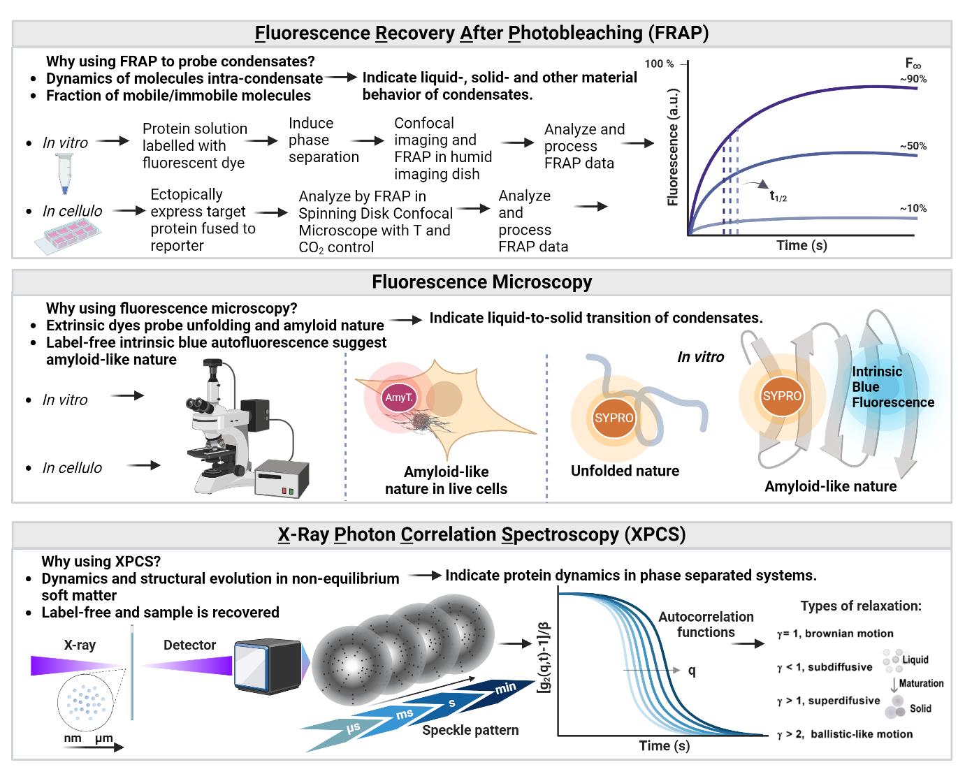
Biophysical methods to characterize biomolecular condensates. Top: Experiments using fluorescence recovery after photobleaching (FRAP) probe the mobility of proteins, RNAs, or other molecules composing the dense phase. The fraction of mobile molecules corresponds to the plateau fluorescence (F∞), and the kinetics of recovery are extracted from the half-time of maximum recovery (t1/2). These FRAP parameters are crucial to probe the material state of condensates that can behave as liquids, gels, soft glasses, and solids. Middle: Fluorescence microscopy approaches can inform on the structure of solid-like condensates. For example, SYPRO orange binds to hydrophobic residues exposed to solvent, indicating protein unfolding. AmyTracker 680 probes cross-β structures indicative of amyloid fold. Bottom: XPCS is a coherent scattering technique that probes dynamics in non-equilibrium systems. Monitoring the dynamics during LLPS is important to determine the biomolecular condensate state and droplet fluidity. Figure created in BioRender.com.
Background
The aggregation of the cellular prion protein (PrPC; Uniprot ID P04156) into the pathological scrapie PrP (PrPSc) leads to the development of prion diseases, including Creutzfeldt–Jakob disease in humans, and other fatal neurodegenerative disorders, with average survival time of one year after diagnosis, depending on the disease subtype. It is crucial to understand the mechanism by which PrPC, a monomeric protein that is ~50% disordered (N-terminal domain; residues 23–120) and ~50% globular (C-terminal domain; 120–230), misfolds into amyloids—highly ordered multimers enriched in cross-beta sheet structure—that are protease-resistant (PrPSc) and deposit in the brain (reviewed in [1]). In addition to classical theories of amyloid formation, a non-canonical pathway of misfolding seems to involve protein monomers or multimers in metastable biomolecular condensates, which are protein-rich membranelles assemblies [2,3]. Biomolecular condensates are formed by liquid-liquid phase separation and are driven by proteins enriched in intrinsic disorder and prion-like domains or low complexity sequences, as polar and aromatic residues establish multivalent weak intermolecular interactions that trigger condensation (reviewed in [4,5]).
Condensates display a myriad of functions across different cellular compartments. For example, cytosolic Tau condensates on the microtubule surface are suggested to regulate the movement of motors (reviewed in [6]), Golgi matrix proteins (e.g., Golgins and GRASPS) are suggested to organize the structure of Golgi by their phase separation property (reviewed in [7]), and nucleoid-associated proteins of E. coli compact DNA via phase separation, organizing sub-domains in nucleoids [8]. To understand the role of protein phase separation in cellular outcomes, as well as its relevance to aggregate formation, in vitro reconstituted systems that monitor protein dynamics within condensates, in combination with in cellulo approaches where condensation can be manipulated and quantitatively assessed, are required. Fluorescence recovery after photobleaching (FRAP) has become one of the most useful techniques to quantify the mobile vs. immobile fractions of biomolecules and their exchange between light and dense phases [9,10].
Here, we describe a systematic method to analyze the dynamics of condensates using the full-length PrP as a model. We have recently shown that the full-length PrP forms condensates in response to copper ions in vitro and at the cell–cell interface of live cells exposed to exogenous Cu2+. We first provide a standardized protocol using X-ray photon correlation spectroscopy (XPCS), a synchrotron technique that uses coherent X-rays to resolve the collective dynamics in concentrated protein systems. Because the dynamics of phase-separated systems display non-equilibrium behavior with length scales ranging from nanometers to microns and timescales from microseconds to minutes, XPCS can provide unique insights into biomolecular dynamics and condensate fluidity. Next, we detail strategies using fluorescence microscopy to gain insights into the folding state of proteins in condensates, utilizing extrinsic fluorescence such as SYPRO and AmyTracker 680 that probe unfolding and amyloids. Finally, we describe in vitro FRAP-optimized protocols to characterize reconstituted condensates using recombinant proteins fused to fluorescent reporters (e.g., Alexa 647). For FRAP in cells, we expressed PrPC fused to the enhanced yellow fluorescent protein (EYFP) in HEK293 and monitored FRAP dynamics upon exposure to copper ions in cell media. Using the combination of the three strategies detailed herein enables robust characterization of the biophysical properties and nature of phase-separated states.
Materials and reagents
Biological materials
1. Proteins:
a. Recombinant full-length murine prion protein (rPrP, residues 23–231) without any tag. PrP has an intrinsic ability to coordinate divalent transition metals in the octapeptide region (also termed octarepeats, OR) that we take advantage of to purify using Ni2+-affinity chromatography (explained in Section C) [11]. Mouse PrP has five ORs that can bind up to 4 copper ions, and two additional His in the N-terminal domain can also bind Cu2+, making it six sites for Cu2+
Note: Recombinantly expressed PrP (rPrP) at 70–100 μM is stored in low protein binding microcentrifuge tubes in ultrapure H2O at -20 °C for up to 6 months. We found that rPrP protein stability and solubility as well as secondary and tertiary structures are maintained using these conditions. In addition, rPrP does not phase-separate in H2O; checking this is essential, as LLPS-forming proteins cannot be stored in a condition where phase separation is favored.
b. rPrP labeled with Alexa Fluor 647 (Alexa Fluor® 647 carboxylic acid, succinimidyl ester) by formation of a stable dye-protein conjugate, as the reactive dye contains a succinimidyl ester moiety that reacts with primary amines of proteins such as the N-terminus and the side-chain of lysine residues (Thermo Fisher, catalog number: A20173) (see [12] for the labeling procedure and consult the manufacturer’s manual)
2. Plasmids:
a. pET-41, in which mouse PrP cDNA (corresponding to amino acid residues 23–230, mature protein) was cloned into NdeI and HindIII sites (original HisTag in the plasmid was removed) for expression in Escherichia coli (refer to Section A)
b. pEYFP-N1 for mammalian expression of PrPC-EYFP-GPI (kindly gifted by Marilene H. Lopes, USP, Brazil) (refer to Section J)
c. pCR3-EYFP-GPI (DAF) for mammalian expression of YFP-GPI (kindly gifted by Daniel Legler, Universität Konstanz, Germany) (refer to Section J)
3. Human embryonic kidney cell line (HEK293 cells) (ATCC, CRL-1573) (refer to Sections J, K, L, and N)
4. Escherichia coli BL21 (DE3) (Thermo Scientific, catalog number: EC0114) (refer to Section A)
Reagents
1. Ultrapure water, treated by reverse osmosis, filtered, and deionized (resistivity of 18.2 MΩ·cm and pH 6.9 at 25 °C)
2. Copper (II) chloride dihydrate (CuCl2·2H2O) (Sigma-Aldrich, catalog number: 307483)
3. 30% (w/v) hydrogen peroxide (H2O2) (Millipore, catalog number: 88597)
4. 4-(2-Hydroxyethyl)piperazine-1-ethanesulfonic acid (HEPES) (C8H18N2O4S) (Sigma-Aldrich, catalog number: V900477)
5. Potassium chloride (KCl) (Sigma-Aldrich, catalog number: P3911)
6. Potassium hydroxide (KOH) (Sigma-Aldrich, catalog number: 484016)
7. Sodium chloride (NaCl) (Sigma-Aldrich, catalog number: S1679)
8. Calcium chloride dihydrate (CaCl2·2H2O) (Sigma-Aldrich, catalog number: V900269)
9. Magnesium chloride hexahydrate (MgCl2·6H2O) (Sigma-Aldrich, catalog number: M2670)
10. Polyethylene glycol (PEG) 4000 (Sigma-Aldrich, catalog number: 81240)
11. Alexa Fluor® 647 Protein Labeling kit (Thermo Fisher, catalog number: A20173)
12. Hydrochloric acid (HCl) (Sigma-Aldrich, catalog number: 30721)
13. Sodium hydroxide (NaOH) (Sigma-Aldrich, catalog number: S5881)
14. Phosphate-buffered saline (PBS) (Thermo Fisher, catalog number: 10010001)
15. Recombinant PrP expression and purification (Sections B and C)
a. 2-amino-2-(hydroxymethyl)-1,3-propanediol (Tris) (C4H11NO3) (Sigma-Aldrich, catalog number: 252859)
b. Ethylenediaminetetraacetic acid (EDTA) (C10H14N2Na2O8·2H2O) (Sigma-Aldrich, catalog number: E4884)
c. Disodium hydrogen phosphate (Na2HPO4) (Sigma-Aldrich, catalog number: S9763)
d. α-D-Glucopyranosyl β-D-fructofuranoside (sucrose) (C12H22O11) (Sigma-Aldrich, catalog number: S8501)
e. Lysozyme from chicken egg white (Sigma-Aldrich, catalog number: L6876)
f. CelLytic B cell lysis reagent (Sigma-Aldrich, catalog number: B7435)
g. Sodium dihydrogen phosphate (NaH2PO4) (Sigma-Aldrich, catalog number: S0751)
h. UltraPure guanidine hydrochloride (CH6ClN3) (Invitrogen, catalog number: 15502016)
i. 1,3-Diaza-2,4-cyclopentadiene (imidazole) (C3H4N2) (Sigma-Aldrich, catalog number: I202)
j. Agar (Becton Dickinson Bioscience, catalog number: 214010)
k. Luria-Bertani (LB) broth (Becton Dickinson Bioscience, catalog number: 244620)
l. Super optimal broth (SOC) (Sigma-Aldrich, catalog number: S1797)
m. Phenylmethanesulfonyl fluoride (PMSF) (C7H7FO2S) (Sigma-Aldrich, catalog number: P7626)
n. HisTrap HP, 5 mL (Cytiva, catalog number: 17524802)
o. SnakeSkin dialysis tubing 10 K MWCO (Thermo Scientific, catalog number: 68100)
p. Triton X-100 (Sigma-Aldrich, catalog number: X100)
q. Colloidal Coomassie G-250 stain for protein polyacrylamide gels (Bio-Rad, catalog number: 1610803)
16. Media for cell culture (Sections J, L, K, and N)
a. Dulbecco’s modified Eagle’s medium (DMEM) (Sigma-Aldrich, catalog number: D5546)
b. Fetal bovine serum (FBS) (Gibco, catalog number: A5670801)
c. Penicillin-Streptomycin 100× (Sigma-Aldrich, catalog number: P4333)
17. Reagents for transfection for in cellulo FRAP experiments (Sections J–L)
a. Opti-MEM I (Gibco, catalog number: 31985062)
b. Lipofectamine 2000 (Invitrogen, catalog number: 11668027)
18. Extrinsic dyes for fluorescence microscopy (Sections H and N)
a. SYPRO orange (5,000× stock in DMSO) (Sigma-Aldrich, catalog number: S5692)
b. AmyTracker 680 (Ebba Biotech AB)
19. Standard for calibration of q-angle for XPCS experiments (Sections E and F)
a. Silver(I) behenate (Thermo Scientific Chemicals, catalog number: 15452307)
Solutions
1. STE buffer (see Recipes)
2. Buffered sucrose (see Recipes)
3. Buffer A (denaturing buffer pH 8.0) (see Recipes)
4. Buffer B (refolding buffer pH 8.0) (see Recipes)
5. Elution buffer pH 5.0 (see Recipes)
6. 2× Physiological-like buffer (PhysB) pH 7.2 (see Recipes)
7. CuCl2, 0.1 M (see Recipes)
8. 3% (or 0.88 M) H2O2 (see Recipes)
9. rPrP sample (see Recipes)
10. rPrP+CuCl2 sample (see Recipes)
11. rPrP+CuCl2+H2O2 sample (see Recipes)
12. Media for cell culture (complete DMEM) (see Recipes)
Recipes
1. STE buffer, pH 8 (100 mL)
| Reagent | Final concentration | Quantity or Volume |
|---|---|---|
| Tris | 50 mM | 0.6056 g |
| NaCl | 10 mM | 0.0584 g |
| EDTA | 5 mM | 0.1861 g |
a. Dissolve the solids in ~80 mL of ultrapure H2O and stir until completely dissolved using a magnetic stirrer.
b. Monitor the pH of the solution (it should be ~7.0–7.5) and adjust to 8 by carefully adding NaOH.
c. Adjust the final volume to 100 mL.
d. Filter-sterilize the solution using a 0.22 μm syringe filter.
e. Store the prepared buffer at 4 °C for up to 1 month.
Note: It is recommended to always use freshly prepared buffers to ensure optimal performance.
2. Buffered sucrose, pH 7.2 (50 mL)
| Reagent | Final concentration | Quantity or Volume |
|---|---|---|
| Na2HPO4 | 20 mM | 0.14196 g |
| NaCl | 20 mM | 0.0292 g |
| EDTA | 5 mM | 0.0931 g |
| Sucrose | 25% (m/v) | 12.5 g |
a. Dissolve the solids in ~30 mL of ultrapure H2O and stir until completely dissolved using a magnetic stirrer.
b. Monitor the pH of the solution (it should be ~7.5–8.0) and adjust to 7.2 by carefully adding HCl.
c. Adjust the final volume to 50 mL with ultrapure H2O.
d. Store the prepared buffer at 4 °C for up to 1 month.
Note: Filtration is not necessary for this buffer due to the high concentration of sucrose, which increases viscosity. Ensure the solution is fully homogeneous and all components are completely dissolved before verifying the pH.
3. Buffer A (denaturing buffer) pH 8.0 (500 mL)
| Reagent | Final concentration | Quantity or Volume |
|---|---|---|
| Ultrapure guanidine | 6 M | 286.59 g |
| Tris | 10 mM | 0.6056 g |
| Na2HPO4 | see note* | 6.7241 g |
| NaH2PO4 | see note* | 0.3184 g |
a. Dissolve Na2HPO4 and NaH2PO4 in ultrapure water and stir until completely dissolved using a magnetic stirrer.
b. Add Tris to the solution and continue stirring until fully dissolved.
c. Add ultrapure guanidine hydrochloride (GdnHCl) and continue stirring until the powder is completely dissolved.
d. Monitor the pH of the solution. If necessary, adjust the pH carefully to 8.0 using HCl or NaOH.
e. Adjust the final volume to 500 mL with ultrapure water.
f. Filter-sterilize the solution using a 0.22 μm syringe filter to ensure sterility.
g. Store the prepared buffer at 4 °C for up to 1 month.
Notes:
1. Ultrapure guanidine (purity ≥99%) is required to avoid impurities that could interfere with the protein purification process.
2. Guanidine is highly hygroscopic and contributes significantly to the final volume.
*Note: Sodium phosphate buffer (monobasic + dibasic) has a final concentration of 100 mM.
4. Buffer B (refolding buffer) pH 8.0 (600 mL)
| Reagent | Final concentration | Quantity or Volume |
|---|---|---|
| Tris | 10 mM | 0.7268 g |
| Na2HPO4 | see note* | 8.0662 g |
| NaH2PO4 | see note* | 0.3815 g |
a. Dissolve Na2HPO4 and NaH2PO4 in ultrapure water and stir until completely dissolved using a magnetic stirrer.
b. Add Tris to the solution and continue stirring until fully dissolved.
c. Monitor the pH of the solution. If necessary, adjust the pH carefully to 8.0 using HCl or NaOH.
d. Adjust the final volume to 600 mL with ultrapure water.
e. Filter-sterilize the solution using a 0.22 μm syringe filter to ensure sterility.
f. Store the prepared buffer at 4 °C for up to 1 month.
*Note: Sodium phosphate buffer (monobasic + dibasic) has a final concentration of 100 mM.
5. Elution buffer pH 5.0 (500 mL)
| Reagent | Final concentration | Quantity or Volume |
|---|---|---|
| Imidazole | 500 mM | 17.02 g |
| NaH2PO4 | 100 mM | 6.0 g |
a. Dissolve NaH2PO4 in ultrapure water and stir until completely dissolved using a magnetic stirrer.
b. Add imidazole to the solution and continue stirring until fully dissolved.
c. Monitor the pH of the solution using a calibrated pH meter. If necessary, adjust the pH carefully to 5.0 using HCl or NaOH.
d. Adjust the final volume to 500 mL with ultrapure water.
e. Filter-sterilize the solution using a 0.22 μm syringe filter to ensure sterility.
f. Store the prepared buffer at 4 °C for up to 1 month.
Note: A significant volume of HCl may be required to reach this pH due to the buffering capacity of imidazole.
6. 2× Physiological-like buffer (PhysB) pH 7.2 (100 mL)
| Reagent | Final concentration (2×) | Quantity or Volume |
|---|---|---|
| HEPES | 20 mM | 0.4766 g |
| KCl | 240 mM | 1.7894 g |
| NaCl | 10 mM | 0.5844 g |
| CaCl2·2H2O | 300 μM | 0.0441 g |
| MgCl2·6H2O | 10 mM | 2.033 g |
| PEG 4000 | 120 mg/mL | 12 g |
| Ultrapure H2O | n/a | to 100 mL |
| Total | n/a | 100 mL |
a. Dissolve the solids in ~80 mL of ultrapure H2O and stir until complete dissolution using a magnetic stirrer.
b. Monitor the pH of the solution (should be acidic, ~5.5) and adjust to 7.2 by carefully adding KOH flakes (do not use NaOH since K+ is prevalent over Na+ in the cellular milieu; see Theillet et al. [13]).
c. Complete the volume to 100 mL.
d. Filter-sterilize using a 0.22 μm syringe filter.
e. Store at 4 °C for up to 1 month or freeze at -20 °C for up to 6 months.
f. Equilibrate the buffer for at least 30 min at room temperature before preparing samples for experiments.
7. CuCl2 0.1 M
| Reagent | Final concentration | Quantity or Volume |
|---|---|---|
| CuCl2·2H2O | 100 mM | 0.85 g |
| Ultrapure H2O | n/a | 49.1 mL |
| Total | n/a | 50 L |
a. Using a CuCl2 powder stored in a sealed container kept inside a desiccator (hygroscopic), weigh the corresponding amount.
b. Completely dissolve the CuCl2 powder.
c. Filter-sterilize and keep at room temperature.
8. 3% (or 0.88 M) H2O2
| Reagent | Final concentration | Quantity or Volume |
|---|---|---|
| Ultrapure H2O | n/a | 450 μL |
| 8.8 M H2O2 | 0.88 M | 50 μL |
| Total | n/a | 500 μL |
Add components in this order in a microcentrifuge tube (1.5 mL capacity).
Note: H2O2 decomposes quickly; make this diluted solution just before preparing the sample. Once open, keep the 30% w/v H2O2 stock container at 4 °C for up to 6 months.
9. rPrP sample
| Reagent | Final concentration | Quantity or Volume |
|---|---|---|
| Ultrapure H2O | n/a | 71 μL |
| 2× physiological buffer (Recipe 6) | 1× | 250 μL |
| rPrP 70 μM | 25 μM | 179 μL |
| Total | n/a | 500 μL |
Add components in this order in a low protein binding microcentrifuge tube.
10. rPrP+CuCl2 sample
| Reagent | Final concentration | Quantity or Volume |
|---|---|---|
| Ultrapure H2O | n/a | 21 μL |
| 2× Physiological buffer (Recipe 6) | 1× | 250 μL |
| rPrP 70 μM | 25 μM | 179 μL |
| CuCl2 2 mM | 200 μM | 50 μL |
| Total | n/a | 500 μL |
Add components in this order in a low protein binding microcentrifuge tube.
11. rPrP+CuCl2+H2O2 sample
| Reagent | Final concentration | Quantity or Volume |
|---|---|---|
| Ultrapure H2O | n/a | 15.3 μL |
| 2× Physiological buffer (Recipe 6) | 1× | 250 μL |
| rPrP 70 μM | 25 μM | 179 μL |
| CuCl2 2 mM | 200 μM | 50 μL |
| H2O2 (3% w/v or 0.98 M) | 10 mM | 5.7 μL |
| Total | n/a | 500 μL |
Add components in this order in a low protein binding microcentrifuge tube.
Note: H2O2 decomposes quickly. Therefore, to have a 3% w/v (or 0.88 M) H2O2 solution, make a 1:10 dilution of 30% w/v H2O2 in ultrapure H2O just before preparing the sample (e.g., 50 μL of H2O2 + 450 μL of H2O) (Recipe 8). Once open, keep the 30% w/v H2O2 stock container at 4 °C for up to 6 months.
12. Media for cell culture (complete DMEM)
| Reagent | Final concentration | Quantity or Volume |
|---|---|---|
| DMEM | n/a | 445 mL |
| FBS | 10% | 50 mL |
| Penicillin/Streptomycin 100× | 1% | 5 mL |
| Total | n/a | 500 mL |
Filter-sterilize using a 0.22 μm membrane, store at 4 °C, and prewarm at 37 °C before culturing HEK293 cells.
Laboratory supplies
1. XPCS measurements:
a. Silanized quartz capillary, 1.5 mm outer diameter, wall thickness 0.01 mm (Hampton Research, catalog number: HR6-128)
b. Disposable syringe, 1 mL
c. 1.5 mL microcentrifuge protein LoBind tubes (Eppendorf, catalog number: 0030108116)
2. Imaging chambers:
a. 35 × 10 mm diameter with a hole punched and 1.33 cm2 area glass coverslip (SPL, catalog number: 200350)
b. μ-slide 8-well confocal slides with lid (Ibidi, catalog number: 80806-90)
c. Coverslips #1 thickness size 22 × 22 mm (Knittel glass, catalog number: VD12222Y100A), microscope slides size 76 × 26 mm (Knittel glass, catalog number: VA21100001FKB), and double-sided tape (3-M Scotch 665-C, 19 mm × 32.9 m)
Equipment
1. XPCS beamline at a synchrotron facility. We used the Cateretê beamline at the Brazilian Synchrotron Light Laboratory (Sirius) [14]. The beamline parameters of the XPCS experiments are detailed in [12].
2. Confocal line-scanning inverted microscope (Carl Zeiss, model: LSM 710) equipped with a 100× objective (oil-immersion, NA 1.46, Carl Zeiss)
3. Confocal spinning disk inverted microscope (Nikon, model: Eclipse-Ti CSU-X) equipped with a 60× objective (oil-immersion, 60×, plan Apo, oil, NA 1.4, Nikon), perfect focus system (PFS), and coupled with temperature, humidity, and CO2 hypoxia incubator (On Stage Incubator, Okolab)
4. Fluorescence microscope (Leica, model: LMD 7) equipped with a 100× objective (Leica Microsystems, model: oil-immersion, NA 1.25)
5. Centrifuge (Hitachi, model: Himac CR22 GII)
6. Centrifuge (Heraeus, model: Megafuge 8R)
7. Spectrophotometer (Shimadzu, model: UV mini-1240)
8. Water bath (Novatecnica)
9. Sonicator (Sonics & Materials, model: VCX 130)
10. Thermal mixer (Eppendorf, model: ThermoMixer F1.5)
11. Incubator shaker (New Brunswick Scientific, model: Excella E24 Incubator Shaker Series)
12. Incubator (Quimis)
13. ÄKTAprimeTM plus (GE Healthcare)
Software and datasets
1. Fiji (Image J) (https://imagej.net/software/fiji/downloads access date July 1, 2024)
2. GraphPad Prism 8.1.1 (https://www.graphpad.com access date July 1, 2024)
3. Excel (Microsoft)
4. XPCS data analysis Python package developed in-house for the calculation of the autocorrelation from the scattering intensity. The software generates multi-tau, one-time, and two-time g2 modes based on the method described by [15]. The temporal autocorrelation function for a set of pixels in a region with an average wavevector q [q = (4π/λ) sin(θ/2) with θ the scattering angle] is given by the one-time correlation
5. SAXS data analysis: SAXS patterns were obtained from the averaged XPCS dataset using the PyFAI software package (https://www.esrf.fr/UsersAndScience/Publications/Highlights/2012/et/et3)
Procedure
A. Transformation of the PrP plasmid and protein expression in E. coli
1. Beforehand, have the following ready:
a. Water bath set at 42 °C.
b. Incubator set at 37 °C.
c. Bacterial shaker set at 37 °C.
d. Ice bath.
2. Clone or obtain the bacterial plasmid for recombinant PrP expression. The gene encoding mature full-length mouse PrP (residues 23–231) was cloned in a pET-41a(+) backbone in which the tags for fusion (GST, 6×His and 8×His) were removed by cloning PrP cDNA into NdeI and HindIII sites.
Note: Any bacterial expression vector can be used to express PrP under the control of an IPTG inducible T7 RNA polymerase promoter. PrP contains five tandem octapeptide repeats that function as an intrinsic affinity tag that can be used for immobilized metal ion affinity chromatography (IMAC). Specifically, the His residues in the octapeptide repeats (PHGGGWGQ) and two additional His in the N-terminal domain are known to coordinate transition divalent metals with high affinity. Therefore, a nickel (Ni2+) HisTrap column is used for protein purification.
3. Thaw a 50 μL aliquot of competent Escherichia coli BL21 (DE3) cells stored at -80 °C on ice. Wait until completely thawed. Do not spin down the cells and gently handle them to retain cell viability. We use the Inoue method (Sambrook and Russel, 2001, protocol 24 [16]; Im et al. [17]) to produce “ultra-competent” bacteria, but any chemically competent cells protocol can be used.
4. Transfer the cells into a 5 mL round-bottom test tube. Add the pET-41-PrP DNA plasmid (up to 25 ng per 50 μL of competent bacterial cells). Use a volume of DNA that does not exceed 5% of the cell volume (up to 2.5 μL). Swirl gently to mix, do not vortex or spin down the cells. Keep the tube on ice for 30 min.
5. Proceed with the heat shock, placing the tube in a pre-heated 42 °C water bath for exactly 90 s.
6. Immediately transfer the tubes to an ice bath, cooling down the cells for 5 min.
7. Add 800 μL of SOC media to each tube and incubate at 37 °C for 45 min in a shaker at 100 rpm.
8. Plate onto 10 cm solid LB agar plates containing 50 μg/mL kanamycin. Approximately 100 μL is sufficient for plating from a miniprep DNA, but we also centrifuge the remaining volume (6,000× g for 3 min) and resuspend in 100 μL of SOC to plate in an additional plate.
9. Incubate the plates at 37 °C overnight in a bacterial incubator. Plates are kept upside down to prevent condensation onto the agar’s surface.
10. Pick a colony from the agar plate using a 200 μL pipette tip. Inoculate 50 mL of LB media with 50 μg/mL kanamycin in a 250 mL Erlenmeyer flask, placing the tip inside.
11. Incubate at 37 °C in a shaker at 250 rpm overnight.
12. On the following morning, transfer 40 mL of the bacterial culture to 800 mL of LB (5% of initial culture) with 50 μg/mL kanamycin in a 2 L Erlenmeyer flask.
13. Monitor the optical density (OD) at 600 nm using a spectrophotometer until the OD600nm reading reaches 0.5–0.6. Then, immediately add 0.5 mM IPTG (400 μL of IPTG using a 1,000× stock solution).
Note: Separate a 100 μL aliquot of the culture before the addition of IPTG in a microcentrifuge tube. Spin down for 30 s at 6,000× g, discard the supernatant, and resuspend the pellet in 30 μL of 5× SDS loading buffer. This aliquot, taken before expression induction, is kept for loading in a 15% SDS-PAGE later.
14. Incubate the culture in a shaker at constant homogenization (250 rpm) at 35 °C overnight (16 h).
Note: On the following morning, save a 25 μL aliquot of the culture after overnight incubation to run in a 15% SDS-PAGE. Process this aliquot as in step A13 (see note). Because the cell mass usually quadruplicates overnight, we use one-fourth of the expression volume to run in the gel, as compared to the uninduced cells aliquot.
15. Harvest the cells by centrifugation at 5,000× g for 15 min at 16 °C. Discard the supernatant. The bacterial pellets can be frozen at -20 °C for up to 1 year.
B. Isolation and solubilization of PrP inclusion bodies
Note: Figure 1 shows an overview of the isolation and solubilization of PrP inclusion bodies.
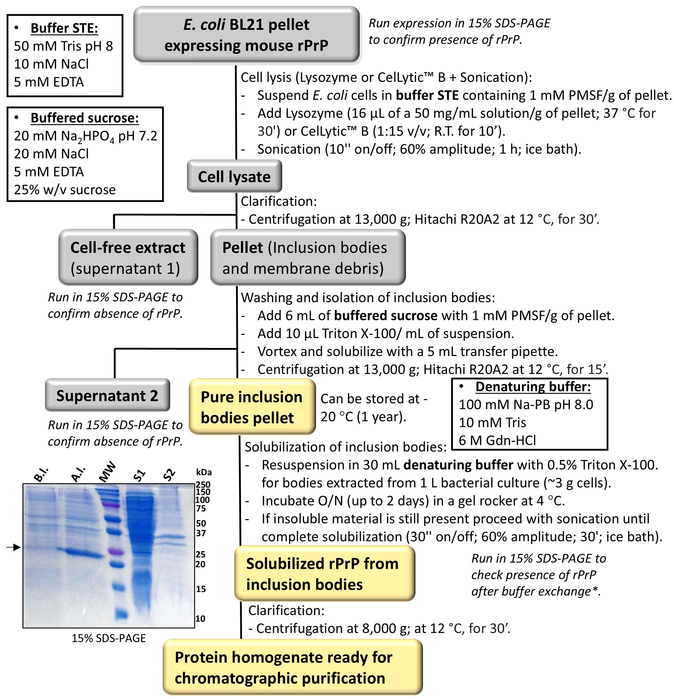
Figure 1. Isolation and extraction of prion protein (PrP) inclusion bodies from E. coli. The flowchart summarizes the steps of inclusion bodies isolation and solubilization by chemical denaturation using guanidine buffer. Recombinant full-length PrP is expressed as insoluble aggregates in the E. coli cytosol within spherical structures known as inclusion bodies. These structures are made of misfolded proteins that interact intra- and intermolecularly in a non-native manner leading to misfolded aggregate formation. Inclusion bodies are usually formed by overexpression of aggregation-prone proteins and/or proteins containing multiple disulfide bridges. The first step of PrP purification consists of the isolation and solubilization of PrP from inclusion bodies. Inset (left): 15% SDS-PAGE of PrP expression in E. coli showing overexpression after induction (A.I.) with IPTG as compared to uninduced cells or before induction (B.I.). Supernatants obtained during the isolation of inclusion bodies were run to show no leakage of PrP that remained in the inclusion bodies’ pellets. S1, supernatant 1. S2, supernatant 2.
1. Beforehand, have the following ready:
a. Set the water bath to 37 °C.
b. Prepare 100 μL of 50 mg/mL lysozyme: weigh 5 mg of lysozyme powder and dissolve with 100 μL of PBS, pH 7.4.
c. Prepare 1 mL of 100 mM PMSF: weigh 0.0174 g of PMSF and add 1 mL of ethanol.
d. Ice bath.
e. Buffers for isolation and solubilization of inclusion bodies: buffer STE, buffered sucrose, and denaturing buffer (see Recipes).
2. In a conical tube containing the bacterial pellet, add 3 mL of buffer A per gram of E. coli pellet and mix using a 5 mL pipettor to form a suspension.
3. Add 100 mM PMSF to the cell suspension to a final concentration of 1 mM (10 μL of 100 mM PMSF per 1 mL of cell suspension).
4. Add 16 μL of 50 mg/mL lysozyme per gram of bacterial pellet and mix thoroughly by pipetting up and down.
5. Incubate the bacterial homogenate in a water bath at 37 °C for 30 min. The mixture will become viscous.
Note: This is the lysis step. Alternatively, CelLytic B (1:15 v/v) can be added to the bacterial suspension instead of lysozyme, followed by incubation at room temperature for 10 min.
6. Sonicate the homogenate using a fine probe: pulse on/off 10 s; amplitude 60% on the ice bath for 1 h. Viscosity should disappear.
7. Transfer the sonicated homogenate into an oak ridge high-speed centrifuge tube (50 mL capacity).
8. Clarify the cell lysate by centrifugation at 13,000× g (10,400 rpm in a Hitachi rotor R20A2) for 30 min at 12 °C.
9. Remove the supernatant and transfer it to a new centrifuge tube. Keep the pellet.
10. Add 3 mL of buffer B per gram of bacterial pellet, mix thoroughly using a micropipette, and vortex to form a suspension.
11. Add 10 μL of 100 mM PMSF and 10 μL of Triton X-100 per milliliter of lysate.
12. Centrifuge at 13,000× g for 15 min at 4 °C.
13. Discard the supernatant and proceed with the denaturation of inclusion bodies in preparation for protein purification.
Note: Alternatively, the pellet containing the isolated inclusion bodies can be frozen at -20 °C for up to 1 year.
14. Resuspend the pellet with 30 mL of denaturing buffer containing 0.5% Triton X-100.
Notes:
1. Adjust the amount of denaturing buffer according to the cell mass. This volume is for inclusion bodies extracted from a 1 L bacterial culture (~3 g of cell mass).
2. Mix the pellet by alternating pipetting up and down with vortexing until only small particles are present; complete homogenization will only take place after overnight incubation.
15. Incubate overnight (up to 2 days) in a gel rocker at 4 °C.
Note: If insoluble material is still present, proceed with sonication: pulse on/off 30 s; amplitude 60% on the ice bath for 30 min. The lysate should become clear.
16. Centrifuge the lysate at 8,000× g for 30 min at 4 °C to remove cell debris. Immediately after centrifugation, transfer the supernatant to a new tube and keep it on ice.
Note: To check the presence of PrP in the solubilized inclusion bodies by SDS-PAGE, it is necessary to remove GdnHCl presence in the denaturing buffer by desalting/buffer exchange. Due to the high ionic strength of GdnHCl, chloride ions disrupt the voltage gradient of the electrophoretic run, and the guanidinium precipitates in the presence of SDS.
C. Recombinant PrP purification
Note: Figure 2 shows an overview of the protein purification steps.
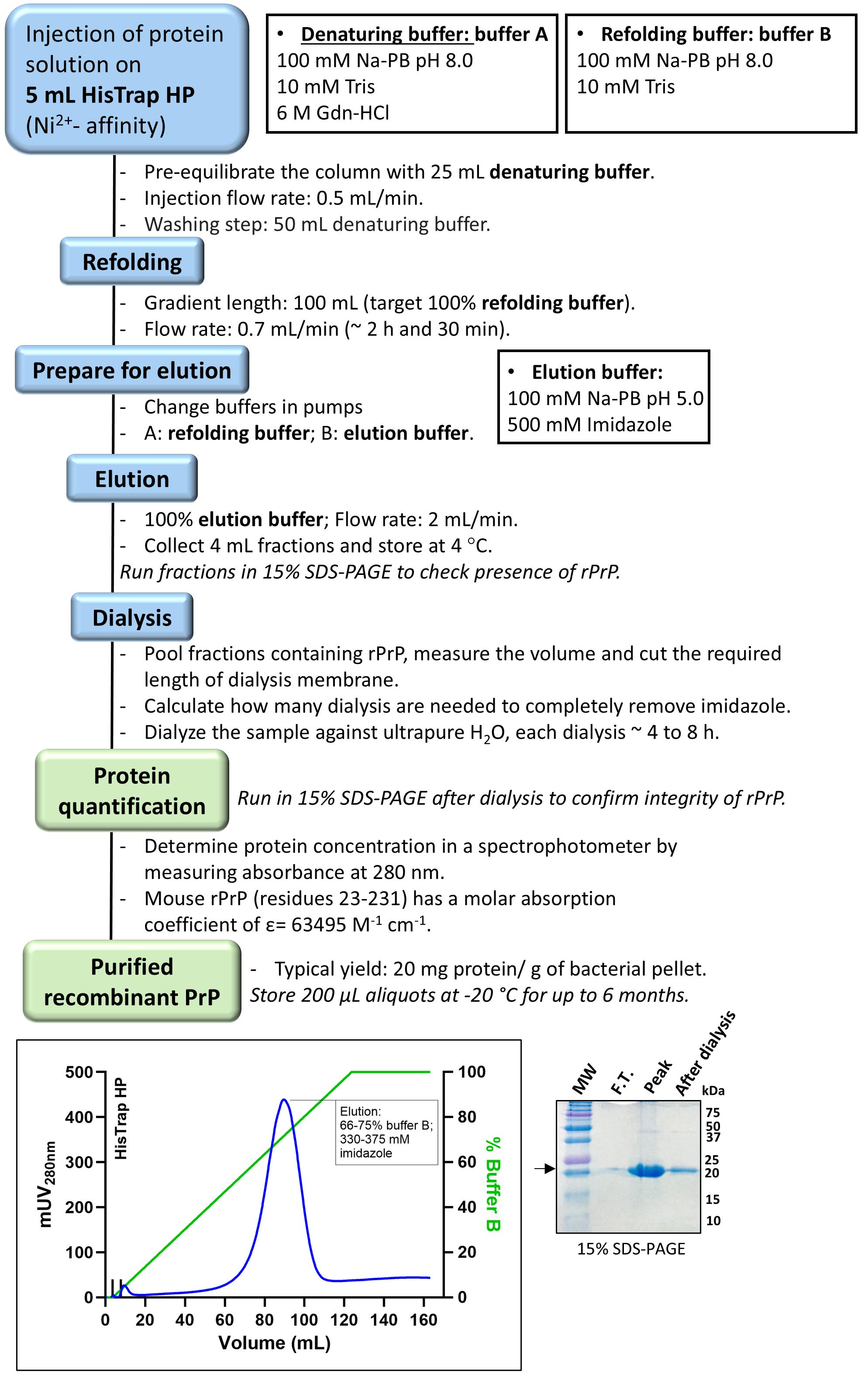
Figure 2. Chromatographic purification of recombinant prion protein (PrP). Flowchart of PrP purification by Ni2+-affinity denaturing chromatography, taking advantage of the intrinsic ability of PrP octarepeats region (59-PHGGGWGQPHGGSWGQPHGGSWGQPHGGGWGQG-90, mouse protein residue numbering) to coordinate divalent transition metal ions, followed by in-column refolding and dialysis against ultrapure water. Inset: Chromatogram of purification and a 15% SDS-PAGE of PrP purification stained with colloidal Coomassie blue. Note the absence of PrP in the flowthrough (F.T.), the presence of PrP in the peak fraction (Peak) as shown by a 23 kDa band, and PrP after buffer exchange (After dialysis). Also, note that a band corresponding to ~46 kDa might be present in the purified fraction corresponding to SDS-resistant PrP dimers.
1. Beforehand, have the following ready:
a. Buffers for Ni2+ affinity chromatography: A (denaturing buffer), B (refolding buffer), and elution buffer (see Recipes).
b. AKTA liquid chromatography system with pumps and tubing in ultrapure H2O.
c. 5 mL HisTrap HP column pre-washed with at least 5 column volumes (CVs) of ultrapure H2O.
2. In the ÄKTA protein purification system, connect the buffer bottles A and B to the respective buffer lines (A1 and B1).
Notes:
1. The end of the buffer lines should be fully submerged in the buffer to avoid air intake.
2. The buffers should be at room temperature before starting the protocol to have the correct pH.
3. Using the ÄKTA menu, prime pumps with the buffers, and make sure any tubing does not show air bubbles or leakage.
4. Connect the HisTrap HP column and equilibrate it with at least 5 CVs of buffer A, or until reaching the baseline of absorbance. Next, auto-zero the UV monitor (absorbance at 280 nm).
Notes:
1. Take note of the conductivity of buffer A for record purposes. The reproducibility of protein purification protocols is directly related to using the correct buffers that should have precise pH, and the conductivity monitor is a good readout of the ionic strength, ensuring that further purification buffers fall within the same range of conductivity.
2. The maximum GdnHCl concentration that HisTrap HP withstands is 6 M, which is the concentration used in buffer A.
5. Load the solubilized inclusion bodies into the 50 mL super loop of ÄKTA.
6. Inject at a slow flow rate of 0.5 mL/min to allow protein binding to the stationary phase.
7. Wash the column with at least 10 CVs of buffer A (denaturing buffer) or until the baselines of absorbance and conductivity are stable.
8. Start the refolding step by setting a gradient from 0% to 100% of refolding buffer (buffer B), with a length of 100 mL and flow rate of 0.7 mL/min. This step takes ~2 h and 30 min. Meanwhile, fill the ÄKTA fraction collector with ice and insert about 20 sterile conical tubes to collect fractions in step C12.
9. Add 4 mL of elution buffer (100 mM sodium phosphate buffer pH 5.0, 10 mM Tris) without imidazole to each tube.
Note: To avoid PrP being eluted in a high concentration that can promote aggregation, we prefill the fraction tubes with elution buffer without imidazole, so the protein is diluted as it drops into the tube.
10. Prepare the ÄKTA system for the elution step. Using the menu, wash the pumps three times with ultrapure H2O.
Note: Because the denaturing buffer has 6 M Gdn-HCl, a throughout cleaning of the pumps is necessary to ensure any residual denaturant is removed.
11. Prime pump A1 with buffer B (refolding buffer) and pump B1 with elution buffer.
12. Elute with a gradient from 0% to 100% elution buffer, with a length of 120 mL and flow rate of 4 mL/min. Collect 4 mL fractions in each tube.
Note: Usually, PrP elutes within 60%–80% of buffer B or 300–400 mM imidazole.
13. Keep the fractions eluted in ice and save 10 μL of each tube to confirm the presence of PrP in the eluted fractions by running a 15% SDS-PAGE.
Notes:
1. Recombinant PrP must be highly purified (≥95%) to avoid interference from possible contaminants.
2. Monomeric rPrP has 23 kDa, and it also forms SDS-resistant dimers that can be visualized in the gel.
14. Pool the fractions containing pure PrP in a single conical tube.
Notes:
1. The fractions can be stored at -20 °C for 1 week before the dialysis step.
2. We do not recommend filtering the PrP solution through a 0.22 μm filter as it tends to stick to the membrane causing protein loss.
15. Add the pooled fractions to a 10 kDa MWCO dialysis membrane. Read the manufacturer user guide for specific instructions.
16. Dialyze the sample against the buffer of choice or ultrapure H2O with a total volume of at least 300 times the volume of the sample. Typically, we use 5 L of ultrapure H2O for 15 mL of pooled fractions, stirring gently for 8–16 h at 4 °C. Repeat dialysis twice more with new ultrapure H2O.
Notes:
1. Because different biophysical/biochemical assays require specific buffers, in our lab, we dialyze PrP against ultrapure H2O. Even though most proteins are not stable in low salt, non-buffered conditions, we established that PrP is well-folded and has α-helical-enriched secondary structure and expected binding properties in H2O. Recover the dialysis membrane, aspirate the solution, and transfer to a new sterile conical tube on ice. Separate a 20 μL aliquot in a microtube to run in a 15% SDS-PAGE to confirm the integrity of rPrP after dialysis.
2. If necessary, the protein solution can be concentrated using 10 kDa cutoff centrifugal filter devices.
17. In a spectrophotometer, add the protein solution to a quartz cuvette and scan from 220 to 320 nm to visualize the spectrum. Measure the absorbance at 280 nm and calculate the concentration using the extinction coefficient for rPrP of 63,945 M-1·cm-1.
Note: The yield of the purification is typically within 15–20 mg of rPrP per gram of bacterial pellet.
18. If the final concentration exceeds 100 μM, dilute the protein solution to 50–70 μM of PrP.
19. Store the sample in 100 μL aliquots in low protein binding microtubes at -20 °C.
Notes:
1. Recombinant PrP can be stored in ultrapure H2O at -20 °C for up to 6 months or at -80 °C for up to 18 months. We recommend periodically collecting circular dichroism and/or fluorescence spectra to probe protein folding after thawing long-stored aliquots.
2. After each purification, proceed with the stripping protocol as recommended by the manufacturer. Next, perform the cleaning protocol to remove ionically bound proteins, precipitated proteins, and hydrophobically bound proteins. Finally, recharge the column with 0.1 M NiSO4, wash extensively with ultrapure H2O, and store the column in 20% ethanol at 4 °C.
D. Recombinant PrP sample preparation
1. Thaw an rPrP aliquot on ice and centrifuge the sample at 8,000× g for 30 min at 4 °C to decant possible aggregates.
2. Transfer the supernatant to a new low binding microcentrifuge tube and determine the protein concentration using an UV-Vis spectrophotometry.
Notes:
1. In our experience, rPrP solutions in ultrapure H2O decrease approximately 2–5 μM after being stored for at least 1 month at -20 °C. This happens because rPrP molecules tend to stick to plastic surfaces and/or small aggregates can be formed during storage. Therefore, it is crucial to determine protein concentration just before conducting experiments.
2. Do not freeze-thaw aliquots. Defrost only the volume needed for experiments. Once thawed, do not freeze the protein solution again.
3. Keep the protein sample on ice to preserve its integrity and molecular stability.
4. Approximately 15 min before preparing rPrP solutions for phase separation assays (see Recipes), equilibrate the rPrP solution at room temperature.
E. X-ray photon correlation spectroscopy assays concomitant to DIC imaging
Notes:
1. Simultaneously with the sample preparation for XPCS, we save an aliquot to perform DIC microscopy to inform whether condensates are present in the sample or not. In addition, after acquiring the XPCS data, we image the sample again to check whether the morphology of condensates changed or if any aggregates were formed.
2. To carry out three different conditions of rPrP samples in triplicate, it is necessary to have approximately 2.5 mg of protein, which is approximately 10% of the yield of rPrP protein purification. Of note, the mouse full-length PrP molecular weight is 23.019 kDa.
1. Condition 1: rPrP protein solution with addition of CuCl2
a. Assemble an imaging chamber using two coverslips fixed on double-sided tape stuck onto a glass slide. The sandwich structure (glass slide–double-sided tape–coverslip) assembles a chamber for sample loading.
b. Turn on the microscope equipped with differential interference contrast (DIC) and a 100× oil immersion objective for DIC (e.g., Leica LMD 7 or Leica TCS SP5).
Notes:
1. Perform Köhler illumination in the brightfield mode to provide homogeneous illumination to your sample and to optimize resolution. Check the microscope manual or consult the core staff for instructions.
2. Make sure that you are using a DIC objective as it is specifically designed with a “strain-free glass” to minimize strain and birefringence, producing accurate images. In addition, check if the required optical accessories are installed in the microscope: condenser Nomarski prism, objective Nomarski prism, polarizer, and analyzer.
c. Dilute the rPrP protein, initially at a concentration of 70 μM, to a final concentration of 25 μM in PhysB pH 7.2 (see Recipes) with addition of 200 μM CuCl2. Prepare a total volume of 500 μL in a low protein binding microtube.
d. Transfer 10 μL of the sample to an imaging microscope slide assembled as in step E1a.
Note: After CuCl2 addition, the rPrP solution will become cloudy, indicating phase separation. Carefully load 490 μL of the rPrP sample into a 1 mL polypropylene syringe, avoiding the formation of air bubbles during the process.
e. Examine the sample under a microscope equipped with differential interference contrast (DIC) (e.g., Leica LMD 7 or Leica TCS SP5).
Notes:
1. In Leica microscopes, by selecting DIC in the software, all optical components will usually be positioned automatically. After placing the specimen on stage, use the knurled wheel below the objective turret or adjust “bias” in the software for fine-tuning the “shear” applied to the light beam by the prism.
2. The DIC image should display a pseudo-3D or shadow-cast appearance with convex-like features or positive bias. Consult literature in DIC and previous DIC images of condensates to familiarize yourself with the technique [18].
f. Adjust the focus and illumination (or gain) as necessary to optimize the visualization of condensates.
g. Acquire 3–5 images of different fields of view of condensates.
Note: Keep track of imaging time as condensates can change morphology over time and wet the surface.
h. Perform the XPCS analysis, as described in Section F.
i. Recover the sample from the syringe, pipette 10 μL in a new imaging chamber, and re-examine the solution under microscopy to detect any changes in the morphology of condensates after exposure to X-ray.
Notes:
1. The parameters of XPCS collection optimized in this protocol have not led to morphological changes in rPrP condensates.
2. Use the same DIC microscopy settings applied in the previous analysis to re-examine the sample.
2. Condition 2: rPrP protein solution
a. Dilute the rPrP protein to a final concentration of 25 μM in 500 μL of PhysB pH 7.2 (see Recipes).
Note: No condensation is observed at this condition (rPrP only at 25 μM in PhysB at room temperature).
b. Follow the same procedures detailed previously in condition 1.
3. Condition 3: rPrP protein solution with the addition of CuCl2 and H2O2 (aggregation over time)
a. Dilute the rPrP protein to a final concentration of 25 μM in 500 μL of physiological buffer pH 7.2 (see Recipes). Add CuCl2 to achieve a final concentration of 200 μM and then add H2O2 to a final concentration of 10 mM.
Note: After CuCl2 and H2O2 addition, the rPrP solution will become very cloudy, indicating phase separation. This sample shows condensates with irregular morphology that over time form aggregates.
b. Follow the same procedures detailed previously in condition 1.
4. Condition 4: Buffer-only control
a. Carefully load 500 μL of physiological buffer pH 7.2 into a 1 mL syringe, avoiding the formation of air bubbles.
b. Perform XPCS measurements.
Note: This step is important to calibrate the system and establish a baseline for comparison with the samples containing rPrP.
F. XPCS measurements
1. Preparation prior to data collection
a. Configure the beamline energy.
b. Adjust the beamline slits to reduce background scattering.
Note: XPCS measurements were performed in small-angle X-ray scattering (SAXS) geometry.
c. Determine the coordinates of the beam center.
d. Calibrate the detector distance in front of the detector tube using silver behenate powder. For long distances, use the detector wagon absolute position encoder, which enables the measurement of translation along the tube.
e. Take exposures of the background and create a mask by outlining regions in the images that should not be included in the autocorrelation (e.g., dead pixels, beam stop, shadows).
2. Collection of XPCS data
a. Load the protein solution in the dry capillary flow cell at 25 °C (Figure 3).
Notes:
1. The typical sample cell for XPCS measurement of protein solution is the temperature-controlled capillary flow cell. The diameter of thin-walled quartz capillaries (10 μm thick) is selected to balance between X-ray scattering and absorption.
2. 500 μL of sample is prepared in a microtube to load 300 μL in the flow cell. If a small amount of protein is available, 400 μL can be prepared. Separate a 10 μL aliquot for DIC visualization before XPCS collection.
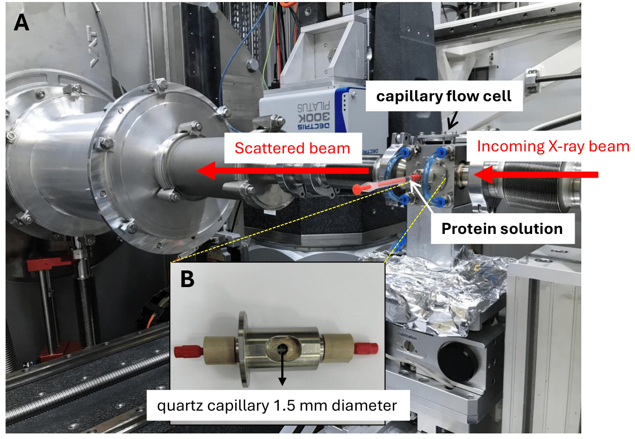
Figure 3. Capillary flow cell for X-ray photon correlation spectroscopy (XPCS) measurements. (A) Capillary flow cell within a thermostatically controlled water bath installed at the experimental hutch at the Cateretê beamline (Sirius, LNLS). The protein solution is introduced into the capillary using a 1 mL syringe. (B) Zoomed view of the capillary adaptor holding a 1.5 mm diameter quartz capillary, 10 μm thick wall.
b. Determine the radiation damage threshold dose value based on any systematic changes in the protein scattering profile [either in the low q range (protein aggregation) or in the high q range (protein degradation)] with increasing X-ray exposure.
Note: If radiation damage is detected in the protein sample, insert an attenuator to reduce the absorbed dose, allowing XPCS measurements below the radiation damage threshold. Radiation damage can be followed by SDS-PAGE analysis of the irradiated samples.
c. Take multiple exposures to define the dynamics time window.
d. Recover the protein sample using a new syringe and load it into a new microtube. Separate a 10 μL aliquot for DIC visualization after XPCS collection.
e. Immediately clean the sample cell rinsing with 10 volumes of ultrapure H2O (3 mL) followed by 5 volumes of 5 M NaCl and 10 volumes of ultrapure H2O. Finally, rinse with 5 volumes of buffer and dry the cell with nitrogen gas flow.
Note: Condensates are sticky and tend to adhere to the capillary wall. We optimized these thorough washing steps including 5 M sodium chloride, as rPrP:CuCl2 condensates are mostly electrostatically driven.
f. Load a fresh protein solution into the flow cell capillary and collect multiple scattering patterns to obtain an XPCS dataset. Check for any time-dependent changes in the shape of the autocorrelation curves.
Note: Users should consult beamline personnel to discuss specific experimental designs and analysis strategies. In addition, many synchrotrons offer workshops and tutorials on XPCS.
3. XPCS data analysis
a. Load the raw data in the XPCS software for calculation of the autocorrelation curves from the X-ray scattering images. Input the parameters related to the experimental conditions (wavelength, sample-to-detector position, beam center, exposure time).
Note: XPCS processing tools/software may be available at the beamline, most of them being custom-made scripts using Python-based graphical user interfaces.
b. Define a region of interest around the scattering region and crop the data to reduce the data size and speed up the analysis (Figure 4).
c. Load the mask created in step F1e.
d. Average the scattering pattern of the XPCS dataset over time, averaging all detector images in the time series for inspection of the data. Any anomalies can be easily identified, such as parasitic scattering from sample cells or no beam, and the dataset can be excluded from the analysis.
e. The SAXS curve from the average scattering pattern can be obtained by azimuthal averaging of the scattering signal using the PyFAI software package.
Note: The SAXS data can be used for the inspection of radiation-induced effects in the protein samples.
f. Before running the XPCS analysis, define the q region and range for the one-time and two-time correlation functions through the parameter’s inner radius of the first ring in pixels, number of rings, and ring thickness in pixels (Figure 4A).
Note: Each individual pixel of the detector contains information about a certain sample’s length scale; however, an individual pixel cannot have enough photon statistics for the XPCS analysis. Selecting a q region and averaging correspondent pixels allow us to improve statistics while maintaining space resolution.
g. Check the sample and beamline stability by inspecting the scattering patterns’ integrated intensity.
Note: The simple inspection of the integrated intensity as a function of time allows the detection of instabilities in the measurement conditions.
h. Run the correlation analysis.
i. To quantify the XPCS, the resulting correlation functions should be fitted with the sum of Kohlrausch–Williams–Watts functions [KWW expression g2(q,t)= 1 + βexp(-2(Γτ)γ)] [19] to extract the parameters β (contrast factor), Γ (relaxation rate), τ (delay time), and γ (KWW exponent) (Figure 4B, C).
Note: The KWW exponent γ will give information about the nature of the relaxation process of the dynamic.
j. Export the results in hdf5 format.
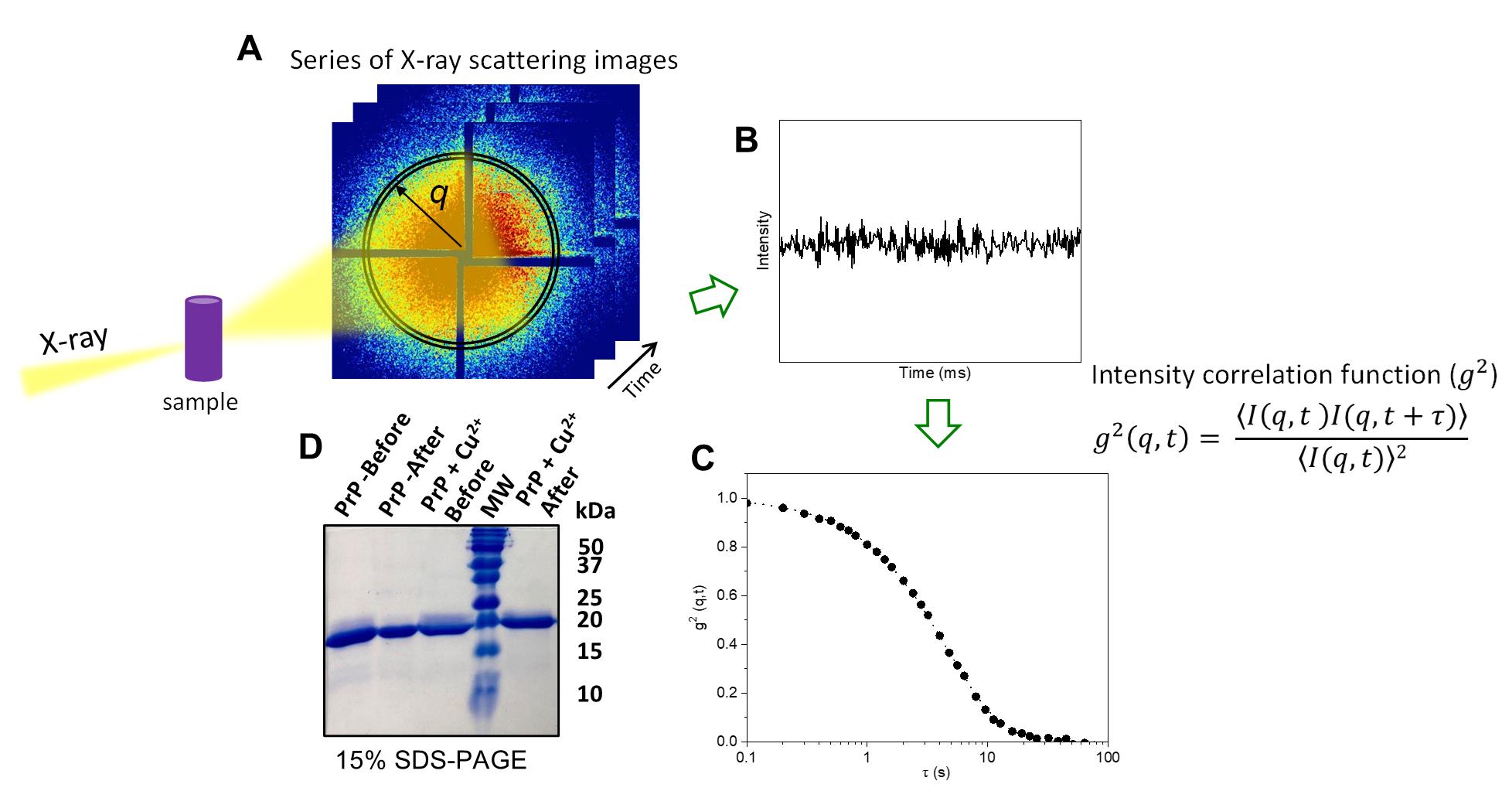
Figure 4. Typical procedure for X-ray photon correlation spectroscopy (XPCS) measurement of protein solutions and data analysis. (A) Multiple scattering patterns are collected during XPCS measurements; images are cropped around a region of interest, and the q region is defined by averaging pixels within the same range of wavevector. (B) The scattering intensity in the q region fluctuates as a function of time due to the changes in the speckle pattern associated with the motion of the scatterers on the sample. (C) Second-order intensity autocorrelation function g2 (q,t) as a function of time delay; the decay characterizes the dynamics of the protein sample. (D) Example of SDS-PAGE analysis to investigate radiation-induced protein cleavage. After optimization of XPCS data collection parameters, samples of prion protein (PrP) (25 μM) in the presence of CuCl2 (200 μM) or not were loaded in the 15% gel before and after irradiation. By comparing the samples, neither PrP nor PrP + Cu2+ showed radiation damage after X-ray exposure.
G. SDS-PAGE analysis following XPCS
1. Prepare samples from each condition to run in a 15% SDS-PAGE gel as described by [20].
2. Stain the gel with colloidal Coomassie blue G-250 [21].
3. Examine the bands on the gel to verify the integrity of the rPrP protein after the XPCS assays.
Note: Proteins can be cleaved by irradiation with X-rays; this is key to ensure that the protein did not suffer radiolysis during exposure to the brilliant light beam, which would compromise XPCS results analysis. rPrP did not suffer radiolysis in all conditions tested, as shown by SDS-PAGE (Figure 4D). A protein sample that underwent radiolysis or chemical degradation would show smaller fragments with lower molecular weights visualized in the SDS-PAGE. Alternatively, radiolysis can be investigated by submitting the sample after XPCS collection to mass spectrometry.
H. Fluorescence microscopy to probe liquid-to-solid transition of condensates
1. Assemble an imaging chamber as described in Section E.
2. Make an intermediate 500× SYPRO orange solution by adding 10 μL of SYPRO (5,000×) to 90 μL ultrapure H2O.
Note: The stock solution of SYPRO orange contains the dye powder solubilized in 100% DMSO. Because of that, we recommend preparing this intermediate SYPRO dilution in H2O to avoid interference of DMSO with condensate characteristics.
3. Premix the rPrP+CuCl2+H2O2 sample in a low protein binding microtube (see Recipes) containing 5 μL of 500× SYPRO orange (final concentration 50×) and incubate for 30 min. The total solution volume is 50 μL, and 20 μL is applied to each chambered well.
4. Image the SYPRO fluorescence in the GFP channel (filter cube with 488 nm excitation and 510 nm emission) or by using the 488 nm laser (emission in the 500–600 nm range) together with DIC or phase contrast to observe the morphology of condensates and/or aggregates.
Notes:
1. It is important to image control samples that do not contain aggregates such as only rPrP and/or rPrP+CuCl2 in which SYPRO orange does not bind.
2. We recommend monitoring the aging of condensates over time by incubating protein samples at increasing time points with SYPRO orange.
3. It is important to image controls of the buffer only and any ligands being tested upon incubation with SYPRO to exclude unspecific binding, as dyes might interact with other components in the protein-containing solution. To note, SYPRO orange has been reported to interact with EDTA, leading to an increase in fluorescence [22].
I. Fluorescence recovery after photobleaching of in vitro rPrP condensates
1. Prepare a 35 mm imaging dish with saturating humidity as in [23]. Briefly, twirl a tissue paper (lint-free) and place it in the outer plastic circumference of the imaging dish. Wet the tissue with 200–300 μL of ultrapure H2O to generate moisture. Do not add an excess of H2O (Figure 5A).
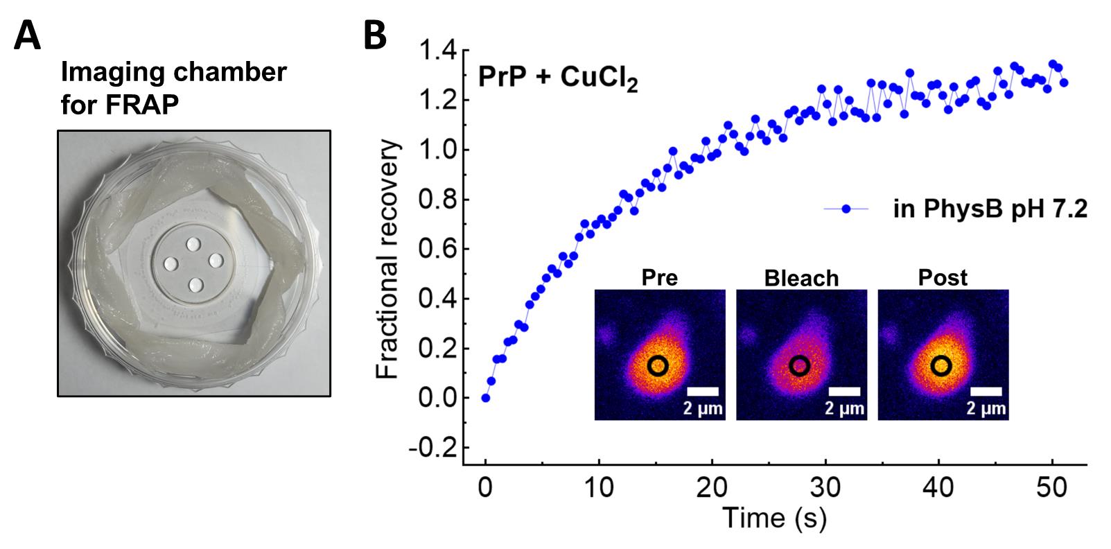
Figure 5. Imaging chamber and example of fluorescence recovery after photobleaching (FRAP) of Cu2+-driven recombinant full-length murine prion protein (PrP) condensates. (A) Imaging chamber for FRAP experiment as described in [23]. To keep the buffer composition and protein concentration unchanged during FRAP acquisition, it is necessary to prepare this humid chamber as evaporation can occur during acquisition. After the addition of ultrapure H2O in the tissue surrounding the coverslip, 3–5 μL of each sample is loaded, and the lid is immediately closed. (B) FRAP recovery of an in vitro prion protein (PrP) condensate formed with 10 μM recombinant PrP (spiked with 0.1% Alexa Fluor 647–labeled rPrP) upon addition of 80 μM CuCl2. The recovery curve of a single condensate is shown after background correction and normalization (Section M). Inset show a PrP:Cu2+ condensate pre-bleaching, immediately after bleaching, and after fluorescence recovery. The experiment was performed 15 min after sample preparation.
2. Prepare 20 μL of unlabeled rPrP samples (see Recipes) containing 0.1% rPrP labeled with Alexa Fluor 647 in a low protein binding microtube.
Note: Adjust the amount of fluorescent protein to be added in the unlabeled protein solution based on the signal-to-noise ratio and background of condensates in the fluorescence images. Typically, 0.1%–1% Alexa 647–labeled protein gives high fluorescence with a good signal-to-noise ratio within the dynamic range.
3. Pipette 5 μL of the LLPS sample and immediately close the dish to prevent evaporation. Incubate for 15 min so the condensates settle to the bottom of the coverslip.
4. Localize the condensates using an oil-immersion 100× objective illuminating with the 633 nm laser line using a fast scan rate (512 × 512-pixel format) to prevent photobleaching and 3× digital zoom to facilitate visualization.
5. Select a field of view with at least two separate condensates with homogeneous fluorescence and diameter of approximately 4–8 μm.
6. Using the ZEN Black software, draw a circular region of interest (ROI) of 1 μm diameter in the center of two condensates, in which one condensate will be bleached and the unbleached one will serve as a reference. Also, draw the same ROI in the background.
Notes:
1. It is important to keep the same ROI size for all condensates and also bleach condensates of similar diameters (4–8 μm, in case of rPrP:Cu2+ samples); inconsistency of these two parameters will directly influence FRAP recovery, making it impossible to compare the results of different conditions.
2. The ROI should be drawn exactly at the center of the condensate to reflect the intra-condensate diffusion.
3. The bleached ROI, unbleached (reference), and background should be taken in every FRAP timelapse. The reference and background will be used for FRAP processing and analysis (Section M).
7. Record 10 frames before bleaching using the 633 nm laser. In order to bleach, proceed using the 405 nm laser (100% intensity, 1,000 iterations), aiming to achieve approximately 50%–90% drop of fluorescence immediately after bleaching.
Note: It is necessary to optimize the number of iterations for bleaching for the first sample, and all parameters should be kept the same. Because Alexa 647 is bright and photostable, we tested and found that 1,000 iterations would be necessary to decrease fluorescence to approximately 50% using the highest energy laser (405 nm) at 100% power and setting pinhole at AU=1. The scan speed of bleach is slowed to yield a pixel dwell of 2.55 μs.
8. Record the recovery after photobleaching for 90–120 s (at a rate of 2 frames/s or frame interval of 0.48 s) until the fluorescence plateaus are reached. Repeat steps I5–8, drawing ROIs to bleach about 5–10 condensates, taking references and backgrounds of each FRAP experiment.
9. Perform quality control of the FRAP experiments collected observing the timelapses and their corresponding curves to spot any artifact. In case the artifacts below occur, data cannot be used.
Note: Aberrant FRAP curves include the following artifacts: (i) focus drifting during acquisition; (ii) condensates that are floating and pass on top of the droplet that has been bleached will cause an abnormal momentaneous increase in the FRAP curve; (iii) a bleached condensate that undergoes fusion during recovery will also have an abnormally higher recovery.
10. Export raw data to Excel for FRAP processing as detailed in Section M. An example of rPrP condensate FRAP is provided in Figure 5B.
J. Transfection of HEK293 cells with PrPC-YFP-GPI or YFP-GPI
1. One day before transfection, pass confluent HEK293 cells by seeding 5 × 10⁴ cells per well in 500 μL of complete DMEM (see Recipes) of an 8-well confocal slide.
Notes:
1. The growth rate of HEK293 cells is usually 24–48 h but also depends on the passage number and growth media. It is necessary to optimize cell concentration according to the growth rate observed in the lab. Cells should be periodically checked for mycoplasma contamination and health observed under phase contrast microscopy, observing the epithelial-like morphology forming a thin monolayer.
2. Use cells with passage no. up to 40. Above that, discard the cells and thaw a new vial that needs to be in culture for three passages before seeding for experiments.
3. We chose HEK293 cells because it is a human cell line that naturally expresses endogenous PrPC (see The Human Protein Atlas, https://www.proteinatlas.org/ENSG00000171867-PRNP/subcellular) and possesses high transfection efficiency. In addition, there are several works that studied PrPC in different epithelial cell models, highlighting the physiological relevance of this system.
2. After 24 h of growth, replace the cell media with 300 μL of Opti-MEM (serum-free and without P/S, at 37 °C) 1 h before transfection.
3. Fifteen minutes before transfection, prepare the transfection mix according to the Lipofectamine 2000 manual. Briefly, prepare two solutions:
a. In a low binding microtube, dilute DNA plasmid (PrPC-YFP-GPI or the YFP-GPI control) in Opti-MEM to 1 μg/well and adjust the volume to 50 μL per well (calculate according to the number of wells). Mix by vortex and spin down.
b. In another low binding microtube, pipette 1 μL of Lipofectamine 2000 in 49 μL of Opti-MEM to 50 μL per well. Mix by gentle tube flickering and pipetting up and down as slowly as possible followed by a spin down.
c. Add the solution from J3a to that of J3b making 100 μL of transfection mix per well, mix by gently flicking the tube (do not vortex), and spin down.
d. Incubate for 10–15 min at room temperature.
4. Pipette off 200 μL of Opti-MEM from each well, leaving 100 μL in each well.
5. Immediately add 100 μL of transfection mix per well in a dropwise manner, swirl the dish, and return cells back to the incubator (37 °C, 5% CO2).
6. After 1 h, carefully pipette cell media off and change media to fresh complete DMEM (500 μL per well).
7. After 48 h post-transfection, proceed to the preparation for live cell imaging.
K. Treatment of transfected HEK293 cells with CuCl2 and preparation for FRAP
1. The cells are in complete DMEM. Change cell media to Opti-MEM (500 μL per well) and place the slide back into the incubator (37 °C; 5% CO2) for 1 h.
Notes:
1. Opti-MEM has a defined composition, as opposed to FBS-containing that varies in composition between lots; to avoid variability during CuCl2 treatment and live cell imaging, we replace growth medium with Opti-MEM.
2. Opti-MEM contains a reduced concentration of phenol red as compared to DMEM (1.1 mg/L vs. 200 mg/L), which is optimal for live cell imaging as phenol red absorbs at 440 nm and can increase background fluorescence, especially of cyan fluorescent proteins.
2. Meanwhile, turn on the spinning disk confocal microscope and pre-equilibrate the stage incubator at 37 °C and 5% CO2 (about 30 min before imaging).
3. After 1 h of cell acclimatation to Opti-MEM, aspirate 5 μL of medium and discard. Apply 5 μL of sterile 30 mM CuCl2 (300 μM Cu2+treated) or 5 μL of H2O (no Cu2+, control). Incubate for 50 min in the incubator (37 °C; 5% CO2).
Note: We collect FRAP data one hour after CuCl2 treatment or not. This short window entails having multiple wells and planning ahead CuCl2 incubation times to coordinate with imaging.
4. In the microscope, put the slide in the equilibrated top stage incubator (37 °C; 5% CO2; humidity control) and wait for 10 min for cells to acclimatize before imaging.
L. Fluorescence recovery after photobleaching of PrPC-YFP-GPI or YFP-GPI at the cell surface
1. Turn on the perfect focus system (PFS), proceed to imaging using a 60× oil immersion objective and the 488-nm laser, and adjust laser power and exposure accordingly. We used 10% laser power and 200 ms exposure.
Notes:
1. It is crucial to have a PFS activated during FRAP acquisition, as focus drifts during the experiment render the data unusable. PFS is a real-time focusing mechanism that automatically corrects for focus drift because of mechanical vibrations or temperature changes.
2. Use low laser power to minimize fluorophore photobleaching and cell toxicity.
2. Precisely focus and find transfected cells showing moderate expression levels.
Draw ROIs of the same size (area: 4.6 μm2; diameter: 2.4 μm) at the cell surface of each cell in the field of view. Draw only one ROI per membrane.
Notes:
1. We observed that cells upon incubation of Cu2+ showed ~2-fold enrichment of PrPC-YFP-GPI at the cell–cell interface [12]. To test whether this enrichment of PrPC-YFP-GPI at the cell–cell interface was driven by condensation, we conducted FRAP. Therefore, we used two FRAP approaches to explore the dynamics of PrPC-YFP-GPI in the plasma membrane of HEK cells: (i) We bleached a ROI at the plasma membrane of a cell facing the extracellular medium, i.e., membranes that do not contact other neighboring cells (isolated), and (ii) we bleached cell–cell interfaces in which membranes of two adjacent cells expressing PrPC-YFP-GPI or YFP-GPI (control) were in contact (Figure 4A).
2. The same ROI size should be used for all FRAP experiments, and only one ROI per cell should be drawn.
3. Do not draw ROIs in cells that are moving or exhibit protrusions.
4. The non-bleached reference and background to subtract FRAP curves will be selected during processing (explained in Section M.
3. Set the bleaching protocol to 100% laser power (488 nm) with two loops (~0.4 s duration).
Note: Photobleaching parameters should be adjusted according to the system examined. We found that this setup gives 50%–70% photobleaching without cytotoxicity. To note, we used the 488 nm laser as the 405 nm can be phototoxic to cells, and UV photobleaching is not recommended.
4. After five initial scans (10% 488 nm), conduct photobleaching (100%, 488 nm) and monitor recovery for 2 min every 200 ms.
Note: Recovery should achieve a plateau and be complete; depending on the system, this time will vary.
5. Proceed collecting FRAP experiments with other fields of view or move to another well (time of treatment with CuCl2 should be 1 h).
Note: Collect FRAP data from at least three independent experiments comprising at least 30 timelapses for every condition as during data processing, quality control will exclude about 10%–20% of data due to cell movements.
6. In addition to saving the FRAP timelapses, save the ROIs with their x and y positions.
M. FRAP data processing and analysis
1. In Fiji (ImageJ), open the FRAP timelapse.
2. Next, open the ROI file: File → Import → Bio-Formats → ROIs.tiff → Open.
3. Transform ROIs’ mask into trackable ROIs that can be saved.
a. Open the ROI manager (Analyze → Tools → ROI manager). Second, using the wand tool, select each ROI and press the Add button in the ROI manager or the shortcut t. This will make a list of all ROIs that are now easily editable.
b. Select all ROIs in the ROI manager menu (Ctrl + A) → More → Save as .zip.
4. Go back to the corresponding FRAP timelapse video and select all in the ROI manager menu. Zoom in to observe each individual ROI before, during bleaching, and during recovery for a quality control englobing the following points:
a. Is it necessary to realign the bleaching spot? If necessary, reposition the bleaching spot as the laser can be slightly shifted in relation to the ROI drawn. It might be worth talking to the microscope facility personnel to calibrate the laser to perfectly match the position of ROIs for further FRAP experiments. However, it is always possible to correct this post-analysis.
b. Does the ROI show unstable pre-bleach fluorescence intensity? In this case, data should not be analyzed.
c. Does the bleached ROI decrease at least 50% of pre-bleach fluorescence? If the bleaching is less than 50%, it is not advisable to proceed with processing.
5. Verify each frame and, if necessary, slightly move ROI across each frame (1–5 pixels) and update in ROI manager. This can happen when minor cell movements take place in the x–y direction.
Note: If cell movements impact fluorescence during recovery, data should not be analyzed.
6. In the main menu: Analyze → Set measurements. Select Area, SD, Mean gray value, and Min/Max.
7. Extract the fluorescence values. Click Measure on the ROI manager menu.
Note: If the bleached ROI position does not need to be repositioned across frames, click in the ROI manager menu More → Multimeasure.
8. Copy data to Microsoft Excel.
9. Repeat steps M4–8 to choose the reference (unbleached ROI) and background fluorescence.
Notes:
1. Do not take reference ROI from the same cell that has been bleached.
2. Reference should have a fluorescence value within the range of pre-bleached fluorescence ROIs.
3. The same size of ROI taken for bleaching should be used to select the reference and the background and extract their values.
10. In Microsoft Excel, background-subtract the value of mean fluorescence intensity of bleached ROI. Do the same for the unbleached ROI (reference).
11. Using background-subtracted intensities, divide the values of the bleached ROI by the reference values. This step corrects the auto-photobleaching due to laser exposure during FRAP acquisition. Using Equation A, F(t) is the background-subtracted fluorescence value of the ROI at a specific time t and CF is the corrected fluorescence intensity.
(A) CF (t) = F(t) of bleached ROI/F(t) of unbleached ROI
12. To determine the mean pre-bleach fluorescence, average the five scans before bleaching:
(B) Average pre-bleach F = Sum of pre-bleach CF/5
13. Normalize the corrected fluorescence intensities to scores from 0 to 1 (Min-max normalization) as in the mathematical formula:
xmaximum = Average pre-bleaching F
xminimum = bleaching F
(A) xt normalized = (xt - xminimum)/(xmaximum - xminimum)
Therefore:
(B) Fractional recovery = (CF(t) – bleaching F)/(Average pre-bleaching F – bleaching F)
14. We make the values 1–100 by multiplying the fractional recovery by 100.
Note: Data analysis of at least 20 ROIs should be carried out.
15. In GraphPad Prism, calculate the mean and error (S.D. or S.E.M.) of the fractional recovery and plot as a function of time.
16. Fit the recovery curve using nonlinear regression and one-phase decay to obtain the half-life of recovery (t1/2). The mobile phase (F∞) is calculated by averaging the plateau recovery fluorescence intensities. Examples of processed FRAP data are included in Figure 6B, C.
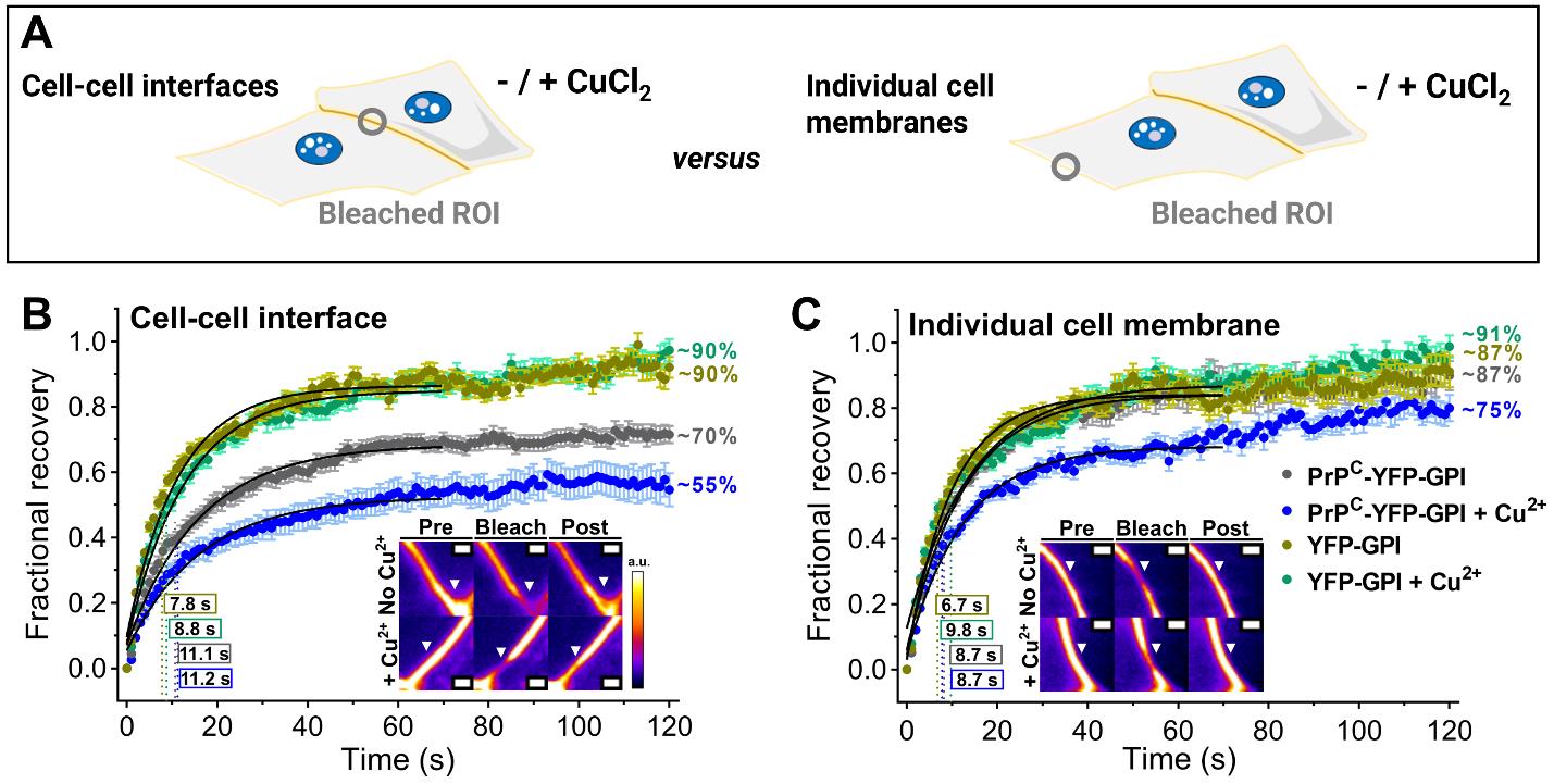
Figure 6. Experimental design data to probe the dynamics of the prion protein (PrPC) in the plasma membrane in response to copper ions by fluorescence recovery after photobleaching (FRAP). (A) HEK293 cells transfected with PrPC-YFP-GPI or YFP-GPI for 48 h were exposed to 300 μM CuCl2 in the cell media for 1 h or not. After that, two different sets of bleaching regions were performed for each of the experimental conditions: (i) bleaching was performed in isolated membranes by drawing a region of interest (ROI) at the cell surface of a membrane facing the cell medium, and (ii) an ROI was drawn at the cell–cell interfaces in which the membranes of two adjacent cells were in contact. FRAP experiments were collected for each condition followed by analysis and processing of data that included background correction and normalization as explained in section M. (B, C) FRAP recovery of PrPC-YFP-GPI or YFP-GPI at cell–cell interfaces vs. individual cell membranes upon Cu2+ treatment or not. Inset show examples of regions before bleaching, directly after bleaching (bleach), and post-fluorescence recovery. Times to half-recovery (t1/2) are indicated inside rectangles, and mobile phases (F∞) in percentage are indicated next to the curves. The experiment was conducted on a confocal spinning disk microscope coupled with a stage-top incubator (37 °C; 5% CO2 and humidity control). ROIs were bleached using a 488 nm laser at 100% laser intensity (2 loops, 0.4 s duration), and a timelapse was collected with frames acquired every 200 ms for 2 min (10% 488 nm laser). Scale bars are 1 μm. Graphs show the mean ± S.E.M. of recovery curves. Panels B and C are reprinted/adapted from Do Amaral et al. [12] Science Advances, DOI: 10.1126/sciadv.adi7347. Some rights reserved; exclusive licensee American Association for the Advancement of Science (AAAS). Distributed under a Creative Commons Attribution Non-Commercial License 4.0 (CC BY-NC 4.0) http://creativecommons.org/licenses/by-nc/4.0/.
N. Live confocal fluorescence microscopy to probe the formation of PrPC-YFP-GPI aggregates by AmyTracker 680
1. Transfect HEK293 cells with PrPC-EYFP-GPI as in Section J.
2. Incubate the cells with 300 μM CuCl2 or not for 3 h, as explained in Section K.
Note: We observed that HEK293 cells transfected with PrPC-EYFP-GPI for 48 h show AmyTracker 680–positive aggregates that co-localize with PrP-EYFP-GPI at the cell surface upon long-term CuCl2 exposure (3 h) in Opti-MEM media.
3. For each well, make an AmyTracker 680 live cell staining solution by adding 0.5 μL of the AmyTracker 680 stock into 500 μL of Opti-MEM (1:1,000). Prewarm this solution for 15 min in a cell culture incubator (37 °C, 5% CO2).
4. Remove the cell culture medium and add the prewarmed AmyTracker 680 staining solution.
5. Incubate for 30 min in a cell culture incubator (37 °C, 5% CO2).
6. Remove the staining solution and replace it with fresh Opti-MEM containing 300 μM CuCl2 or not (depending on the cells’ initial treatment).
7. In a pre-equilibrated (37 °C, 5% CO2) spinning-disk confocal microscope, perform live cell imaging for approximately 1 h using the 488 and 638 nm lasers. In our hands, the optimal settings for both lasers were 10% laser power and exposure of 200 ms.
Note: Image first the 638 nm channel and then the 488 nm. It is advised to image longer wavelengths before those shorter, as more energetic wavelengths are more phototoxic.
8. Image at least three independent biological replicates for each condition.
Note: It is crucial to image controls of AmyTracker 680 in non-transfected cells and cells expressing PrPC-EYFP-GPI only without the influence of any treatment(s) as amyloid dyes might show nonspecific binding to other components. To note, both AmyTracker dyes and thioflavin T (ThT) belong to the class of oligothiophenes. Thioflavin T (ThT) unspecifically bind to nucleic acids. However, thioflavin-S (ThS), another classical amyloid dye, does not bind to single-stranded nucleic acids and nucleic acids containing secondary structures [24]. Therefore, it is key to rule out artifacts caused by nonspecific interactions of fluorescent dyes.
Validation of protocol
This protocol (or parts of it) has been used and validated in the following research article(s):
This protocol has been used and validated in Do Amaral et al. [12]; DOI: 10.1126/sciadv.adi7347 and Do Amaral et al. [25]; DOI: 10.1016/j.bbrc.2025.151489.
Acknowledgments
This work was supported by Coordenação de Aperfeiçoamento de Pessoal de Nível Superior–Brasil (CAPES) (Finance Code 001) (M.J.A.), Fundação de Amparo à Pesquisa do Estado do Rio de Janeiro (FAPERJ), Conselho Nacional de Desenvolvimento Científico e Tecnológico (CNPq), Brazilian Synchrotron Light Laboratory (LNLS) of the Brazilian Ministry for Science, Technology, Innovations and Communications (MCTIC) (CATERETE-20220546), CAPES-PrInt scholarship, grant number 88887.695190/2022-00 (M.J.A.), German Research Society (DFG), priority program SPP2191 (419138680) (S.W.), Helmholtz Association, Institutional funding (S.W.), and Hertie Foundation (P1200002) (S.W.).
Competing interests
There are no competing interests to disclose.
References
- Do Amaral, M. J. and Cordeiro, Y. (2021). Intrinsic disorder and phase transitions: Pieces in the puzzling role of the prion protein in health and disease. Prog Mol Biol Transl Sci. 183: 1–43. https://doi.org/10.1016/bs.pmbts.2021.06.001
- Elbaum-Garfinkle, S. (2019). Matter over mind: Liquid phase separation and neurodegeneration. J Biol Chem. 294(18): 7160–7168. https://doi.org/10.1074/jbc.rev118.001188
- Michaels, T. C. T., Qian, D., Šarić, A., Vendruscolo, M., Linse, S. and Knowles, T. P. J. (2023). Amyloid formation as a protein phase transition. Nat Rev Phys. 5(7): 379–397. https://doi.org/10.1038/s42254-023-00598-9
- Weber, S. C. and Brangwynne, C. P. (2012). Getting RNA and Protein in Phase. Cell. 149(6): 1188–1191. https://doi.org/10.1016/j.cell.2012.05.022
- Boeynaems, S., Alberti, S., Fawzi, N. L., Mittag, T., Polymenidou, M., Rousseau, F., Schymkowitz, J., Shorter, J., Wolozin, B., Van Den Bosch, L., et al. (2018). Protein Phase Separation: A New Phase in Cell Biology. Trends Cell Biol. 28(6): 420–435. https://doi.org/10.1016/j.tcb.2018.02.004
- Mohapatra, S. and Wegmann, S. (2023). Biomolecular condensation involving the cytoskeleton. Brain Res Bull. 194: 105–117. https://doi.org/10.1016/j.brainresbull.2023.01.009
- Mendes, L. F. S., Oliveira, C. G., Simões, K. F., Kava, E. and Costa-Filho, A. J. (2024). Exploring liquid-liquid phase separation in the organisation of Golgi matrix proteins. Biochim Biophys Acta Proteins Proteom. 1872(5): 141029. https://doi.org/10.1016/j.bbapap.2024.141029
- Gupta, A., Joshi, A., Arora, K., Mukhopadhyay, S. and Guptasarma, P. (2023). The bacterial nucleoid-associated proteins, HU and Dps, condense DNA into context-dependent biphasic or multiphasic complex coacervates. J Biol Chem. 299(5): 104637. https://doi.org/10.1016/j.jbc.2023.104637
- Taylor, N. O., Wei, M. T., Stone, H. A. and Brangwynne, C. P. (2019). Quantifying Dynamics in Phase-Separated Condensates Using Fluorescence Recovery after Photobleaching. Biophys J. 117(7): 1285–1300. https://doi.org/10.1016/j.bpj.2019.08.030
- Kenworthy, A. K. (2023). What’s past is prologue: FRAP keeps delivering 50 years later. Biophys J. 122(18): 3577–3586. https://doi.org/10.1016/j.bpj.2023.05.016
- Yin, S. M., Zheng, Y. and Tien, P. (2003). On-column purification and refolding of recombinant bovine prion protein: using its octarepeat sequences as a natural affinity tag. Protein Expression Purif. 32(1): 104–109. https://doi.org/10.1016/s1046-5928(03)00195-5
- Do Amaral, M. J., Mohapatra, S., Passos, A. R., Lopes da Silva, T. S., Carvalho, R. S., da Silva Almeida, M., Pinheiro, A. S., Wegmann, S. and Cordeiro, Y. (2023). Copper drives prion protein phase separation and modulates aggregation. Sci Adv. 9(44): eadi7347. https://doi.org/10.1126/sciadv.adi7347
- Theillet, F. X., Binolfi, A., Frembgen-Kesner, T., Hingorani, K., Sarkar, M., Kyne, C., Li, C., Crowley, P. B., Gierasch, L., Pielak, G. J., et al. (2014). Physicochemical Properties of Cells and Their Effects on Intrinsically Disordered Proteins (IDPs). Chem Rev. 114(13): 6661–6714. https://doi.org/10.1021/cr400695p
- Meneau, F., Passos, A. R., Garcia, P. R. A. F., Vinaches, P., Manoel, L. B., Kalile, T. A., Zerba, J. P., Rodrigues, G. L. M. P., Miqueles, E., Baraldi, G., et al. (2021). Cateretê: the coherent X-ray scattering beamline at the fourth-generation synchrotron facility SIRIUS. Acta Crystallographica Section A. A77: C283–C283. https://doi.org/10.1107/s0108767321093995
- Lumma, D., Lurio, L. B., Mochrie, S. G. J. and Sutton, M. (2000). Area detector based photon correlation in the regime of short data batches: Data reduction for dynamic x-ray scattering. Rev Sci Instrum. 71(9): 3274–3289. https://doi.org/10.1063/1.1287637
- Sambrook, J. and Russell, D. W. (2001). Molecular Cloning: A Laboratory Manual. 3rd ed. New York: Cold Spring Harbor Laboratory Press.
- Im, H. (2011). The Inoue Method for Preparation and Transformation of Competent E. coli: “Ultra Competent” Cells. Bio Protoc. 1(20): e143. https://doi.org/10.21769/bioprotoc.143
- Do Amaral, M. J., Passos, Y. M., Almeida, M. S., Pinheiro, A. S. and Cordeiro, Y. (2023). In Vitro Characterization of Protein:Nucleic Acid Liquid–Liquid Phase Separation by Microscopy Methods and Nanoparticle Tracking Analysis. Methods Mol Biol. 2551: 605–631. https://doi.org/10.1007/978-1-0716-2597-2_37
- Williams, G. and Watts, D. C. (1970). Non-symmetrical dielectric relaxation behaviour arising from a simple empirical decay function. Trans Faraday Soc. 66: 80. https://doi.org/10.1039/tf9706600080
- Laemmli, U. K. (1970). Cleavage of Structural Proteins during the Assembly of the Head of Bacteriophage T4. Nature. 227(5259): 680–685. https://doi.org/10.1038/227680a0
- Dyballa, N. and Metzger, S. (2009). Fast and Sensitive Colloidal Coomassie G-250 Staining for Proteins in Polyacrylamide Gels. J Visualized Exp. 30: e3791/1431. https://doi.org/10.3791/1431
- Kroeger, T., Frieg, B., Zhang, T., Hansen, F. K., Marmann, A., Proksch, P., Nagel-Steger, L., Groth, G., Smits, S. H. J., Gohlke, H., et al. (2017). EDTA aggregates induce SYPRO orange-based fluorescence in thermal shift assay. PLoS One. 12(5): e0177024. https://doi.org/10.1371/journal.pone.0177024
- Hochmair, J., Exner, C., Betzel, C., Mandelkow, E. and Wegmann, S. (2022). Light Microscopy and Dynamic Light Scattering to Study Liquid-Liquid Phase Separation of Tau Proteins In Vitro. In: Protein Aggregation: Methods and Protocols. New York, NY: Springer US. 225–243. https://doi.org/10.1007/978-1-0716-2597-2_15
- Sugimoto, S., Arita-Morioka, K. I., Mizunoe, Y., Yamanaka, K. and Ogura, T. (2015). Thioflavin T as a fluorescence probe for monitoring RNA metabolism at molecular and cellular levels. Nucleic Acids Res. 43(14): e92–e92. https://doi.org/10.1093/nar/gkv338
- Do Amaral, M. J., M., Soares de Oliveira, L. and Cordeiro, Y. (2025). Zinc ions trigger the prion protein liquid-liquid phase separation. Biochem Biophys Res Commun. 753: 151489. https://doi.org/10.1016/j.bbrc.2025.151489
Article Information
Publication history
Received: Oct 24, 2024
Accepted: Mar 6, 2025
Available online: Mar 26, 2025
Published: Apr 20, 2025
Copyright
© 2025 The Author(s); This is an open access article under the CC BY-NC license (https://creativecommons.org/licenses/by-nc/4.0/).
How to cite
Readers should cite both the Bio-protocol article and the original research article where this protocol was used:
- Do Amaral, M. J., Passos, A. R., Mohapatra, S., Freire, M. H., Wegmann, S. and Cordeiro, Y. (2025). X-Ray Photon Correlation Spectroscopy, Microscopy, and Fluorescence Recovery After Photobleaching to Study Phase Separation and Liquid-to-Solid Transition of Prion Protein Condensates. Bio-protocol 15(8): e5277. DOI: 10.21769/BioProtoc.5277.
- Do Amaral, M. J., Mohapatra, S., Passos, A. R., Lopes da Silva, T. S., Carvalho, R. S., da Silva Almeida, M., Pinheiro, A. S., Wegmann, S. and Cordeiro, Y. (2023). Copper drives prion protein phase separation and modulates aggregation. Sci Adv. 9(44): eadi7347. https://doi.org/10.1126/sciadv.adi7347
Category
Biophysics > X-ray crystallography
Biophysics > Microscopy
Biochemistry > Protein > Activity
Do you have any questions about this protocol?
Post your question to gather feedback from the community. We will also invite the authors of this article to respond.