- Protocols

- Articles and Issues
- For Authors
- About
- Become a Reviewer

A Detailed Guide to Recording and Analyzing Arabidopsis thaliana Leaf Surface Potential Dynamics Elicited by Mechanical Wounding
Published: Vol 15, Iss 7, Apr 5, 2025 DOI: 10.21769/BioProtoc.5252 Views: 1495
Reviewed by: Raju MondalAnonymous reviewer(s)
Original research article
The authors used this protocol in:

Sep 2021
Advertisement


Protocol Collections
Comprehensive collections of detailed, peer-reviewed protocols focusing on specific topics


Related protocols
Abstract
Recordings of electric potential changes on plant surfaces have been utilized to identify the components and mechanisms involved in the formation and transmission of systemic signals elicited by stimuli such as herbivory, wounding, or burning. The recorded responses, commonly referred to as slow wave or variation potentials, exhibit striking variability in their waveform. The extent to which this variability is due to differences in experimental procedures or plant biological variability remains unclear. Here, we provide a detailed and robust protocol refined from years of experience in conducting leaf surface potential recordings of Arabidopsis thaliana in response to mechanical wounding. This protocol serves as a comprehensive tutorial covering plant growth, procedures for reproducible mechanical wounding, critical aspects of electrophysiological recordings, and statistical analysis of surface potential recordings. It particularly emphasizes the construction and maintenance of electrodes, placement of the reference or ground electrode, mechanisms for wounding, and data analysis. This protocol aims to promote and facilitate the adoption, standardization, and interoperability of plant surface potential recordings among research groups, thereby increasing the reproducibility and comparability of data within the field.
Key features
• Recording electric potential changes on the petiole of 5-week-old Arabidopsis plants using noninvasive surface electrodes, improving the wounding procedure, reproducibility, and data processing from [1].
• Genotype-independent method for phenotyping, including parallel recordings from multiple plants.
• Guidelines for plant growth conditions, unambiguous leaf assignment by order of emergence, and detailed instructions for electrode fabrication and maintenance.
• Instructions for constructing devices for standardized, reproducible mechanical wounding along with a custom script for unbiased and semi-automated data analysis.
Background
The first known recorded electrical impulses in plants date back to the 19th century from a modified leaf surface of a Venus flytrap (Dionaea muscipula) [2]. Later studies investigated surface potential dynamics in other thigmonastic organs in plants such as Mimosa pudica. Inserted electrode measurements in plants were first performed in the 20th century [3] and, decades later, led to the identification of ion channels as the basis of electrical signals in plants [4]. Modern studies have shown that various environmental stimuli such as light, heat, cold, and wounding trigger electrical signals [5]. Plants can utilize these signals to share information over long distances between organs and to regulate physiological functions [6].
In order to measure electric potential changes in plants, two methods are commonly used: extracellular and intracellular recordings. Although intracellular recordings offer higher precision and cellular resolution, they are typically only effective for short durations due to factors such as cell damage from electrode insertion. Extracellular recordings on the surface of plants are noninvasive, allowing long-term monitoring, but they do not provide information about the electric potential changes of individual cells or specific tissues. Both intracellular and extracellular recordings help identify and monitor diverse electric potential changes, such as action potentials (APs) and slow wave potentials (SWPs). APs are short-lasting, self-propagating electrical signals with a fixed amplitude that can be elicited by stimuli such as cold shock. SWPs are long-lasting electrical signals with variable amplitudes and waveforms that are caused by severe local damage. Unlike APs, SWPs do not self-propagate and require chemical and mechanical signals for generation [7]. The method described here provides detailed instructions for reliably detecting these highly variable changes in plant surface potential.
Materials and reagents
Biological materials
1. Arabidopsis thaliana (L.) Heynh. (Col-0), available from the European Arabidopsis Stock Centre (NASC), the Arabidopsis Biological Resource Center (ABRC), or similar germline resources
Reagents
1. Murashige & Skoog (MS) basal salt mixture, including MES buffer (Duchefa, catalog number: M0254.0050)
2. Low electroendosmosis (LE) agarose (Biozym, catalog number: 840000)
3. Potassium chloride (KCl) (VWR, catalog number: 26764.3)
4. Silver chloride (AgCl) (Sigma-Aldrich, catalog number: 204382-5G)
5. Ethanol (C2H5OH) (Supelco/Merck, catalog number: 1070172511)
6. Sodium hypochlorite (NaOCl) 13% (Fisher Scientific, catalog number: 10691164)
7. Ammonium hydroxide (NH4OH) 25% (Sigma-Aldrich, catalog number: 1336-21-6)
8. DanKlorix® original (2.8 g per 100 mL of sodium hypochlorite) (Office discount, catalog number: 327692)
Solutions
1. 50 mM electrode solution (see Recipes)
2. 5% NaOCl (see Recipes)
3. 70% ethanol (see Recipes)
4. 1/2 MS medium (see Recipes)
Recipes
1. 50 mM electrode solution
Note: To prepare the electrode solution, slowly add AgCl to the dissolved KCl, stirring until undissolved AgCl remains, indicating saturation. Depending on whether you prepare the solution for connecting the electrode to the leaf or for the bath electrode, you need to use 0.8% or 3% LE agarose, respectively.
| Reagent | Final concentration | Quantity or Volume |
|---|---|---|
| KCl | 50 mM | 0.37 g |
| AgCl | n/a | Until saturation is reached |
| MilliQ H2O | n/a | 100 mL |
| Total | n/a | 100 mL |
| LE agarose | 0.8 or 3% (w/v) | 0.8 g or 3 g |
2. 5% NaOCl
Note: This solution has to be prepared freshly before every usage.
| Reagent | Final concentration | Quantity or Volume |
|---|---|---|
| 13% NaOCl | 5% | 3.84 mL |
| MilliQ H2O | n/a | 6.16 mL |
| Total | n/a | 10 mL |
3. 70% ethanol
| Reagent | Final concentration | Quantity or Volume |
|---|---|---|
| Ethanol (absolute) | 70% | 700 mL |
| MilliQ H2O | n/a | 300 mL |
| Total | n/a | 1,000 mL |
4. 1/2 MS medium
Note: To prevent contamination and extend shelf life, autoclave or filter-sterilize the solution. Store at room temperature (RT) if sterile; otherwise, keep at 4 °C and acclimate to RT before use.
| Reagent | Final concentration | Quantity or Volume |
|---|---|---|
| MS including MES buffer | 1/2 strength | 2.6 g |
| MilliQ H2O | n/a | 1,000 mL |
| Total | n/a | 1,000 mL |
Laboratory supplies
1. Pipette tips, 200 μL (Starlab, catalog number: S1113-1206-C)
2. PCR tubes (Sarstedt, catalog number: 72.985.002)
3. Parafilm (Carl Roth, catalog number: H666.1)
4. Forceps (Sigma-Aldrich, catalog number: F4517)
5. Trays (Meyer, catalog number: 749112/74 91 12)
6. Lids (Meyer, catalog number: 749150/74 91 50)
7. Pots 4.5 × 4.5 × 7 cm (Meyer, Göttinger, catalog number: 722001/72 20 01)
8. BP substrate (Baywa, Klasmann-Deilmann, catalog number: 1073986)
9. Vermiculite (Duengerexperte, catalog number: p89)
10. Sand (Lehmann Baustoffe, type: Rheinsand, granulation ≤2 mm)
11. Container to place the pots containing 1/2 MS media for recordings
Equipment
1. Insulating tape (Adam Hall 580813RNB10, Conrad Electronic, catalog number: 5906194000459)
2. Solder (Stannol, model: S-Sn99,3Cu0,7)
3. Soldering iron (Basetech ZD-70D, Conrad Electronic, catalog number: 4064161149202)
4. Banana plug 2 mm (Amazon, catalog number: GST-2.0MM-SCHR)
5. Optical table with sealed holes (Thorlabs, catalog number: B75120A)
6. Silver wire, >99.99% purity, 1 mm diameter (World Precision Instruments, catalog number: AGW4010)
7. Amplifier head stages (NPI Electronic GmbH, model: EXT-02F/2 B)
8. Extracellular amplifier (NPI Electronic GmbH, model: EXT-02F)
9. Digitizer (World Precision Instruments, model: Lab-Trax-4/16, 2016 B016N)
10. Micromanipulator (MM33, 3 Axes, Märzhäuser Wetzlar)
11. Grip wrench (C.K. Tools, catalog number: 000829025)
12. Desiccator (Carl Roth, catalog number: AHL0.1)
13. Microwave
14. Hotplate stirrer (IKA® C-Mag, Sigma-Aldrich, catalog number: Z672351)
15. Emery paper (Bosch Accessories J45 grit 120, Conrad Electronic, catalog number: 3165140678421)
16. 3D-printed grids for leaf wounding (self-printed; the design can be found here)
17. Permanent marker pen (Edding, model: 751)
Software and datasets
1. LabScribe: iWorx v4.345, this license is free to use for research purposes
2. LabView NI (23.1001)
3. R Studio (2023.09.0+463 or younger)
Note: All codes have been deposited toGithub.
Procedure
A. Plant growth (start 6–7 weeks before recordings)
Note: Place a couple of seeds in one pot in case the germination rate is low. At 5 days old, thin the seedlings to leave one plant per pot.
1. Seeding plants
a. Clean all trays and lids with 70% ethanol.
b. Disinfect seeds in a desiccator with DanKlorix®, using the chlorine gas method [8].
c. Prepare the soil by mixing BP substrate, sand, and vermiculite in an 8:1:1 ratio.
d. Add 125 mL of tap water to 500 g of the soil mixture.
e. Microwave for 10 min at 800 W.
f. After cooling down, fill the pots with the soil mixture.
g. Seed the sterilized seeds on the pots filled with room-temperature soil.
h. One plant per pot is needed.
i. Stratify seeds for two days by placing pots containing soil and seeds in a tray closed with a lid at 4 °C.
j. Transfer pots after these two days into the growth chamber.
2. Grow the plants for 5–6 weeks in a growth chamber under short-day photoperiod conditions (10/14 h light/dark cycle) at 22 °C, with 60% humidity, and light intensity of ~120 μmol·m2·s-1. Water when needed.
Note: Avoid overwatering plants to reduce the risk of root anoxia and pest infestations. Older plants should be watered more frequently.
a. Growth under short-day conditions is used to promote vegetative growth and suppress bolting and flowering.
b. Maintaining pest- and pathogen-free conditions is important for plant vigor and ensuring data reproducibility.
c. Space plants at sufficient distances to avoid the leaves touching and to prevent leaf damage (Figure 1A).
d. After 2–3 weeks, gradually remove the tray lid. Start by propping it ajar for a few days to adjust humidity before fully removing it.
3. Counting leaves (ideally in week 4 of growth)
Note: Before counting, each plant should be pre-inspected. Plants showing signs of damage, detached leaves, or growth defaults should be excluded. Leaf 13 is usually found between leaf 8 and 5 (which helps as an orientation).
a. Cotyledons are excluded from counting or numbering.
b. Determine whether the order of leaf emergence is clockwise or counterclockwise (from young to old) by determining the spirality of the plant from the top of the rosette [9].
c. The leaves usually grow at a 137.5° angle, which can be helpful for identifying the next leaf (Figure 1B).
d. Count leaves sequentially in reverse chronological order from the oldest leaf toward the newer leaves (Figure 1C, D).
e. Mark the position of your leaves of interest at the pot using a permanent marker (in our case, 8 and 13; Figure 1E).
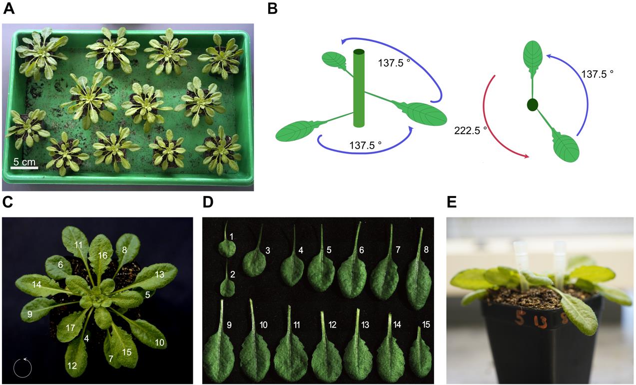
Figure 1. Arrangement and leaf counting of 5-week-old Arabidopsis thaliana for surface potential recordings. (A) Plant arrangement in the tray. Each plant has enough space to avoid contact with others. (B) Schematic drawing of leaf growth and angle. Starting with the third leaf, all subsequent leaves grow at an angle of approximately 137.5°. (C) Rosette of a 5-week-old Arabidopsis. The growth direction is indicated with a circle in the bottom-left corner. Leaves are numbered from oldest to youngest. (D) Single leaves of a 5-week-old Arabidopsis. (E) Example of labeling the leaves of interest (e.g., 13 and 8).
B. Electrode preparation
1. Soldering (Figure 2)
a. Cut segments of silver wire to the desired lengths, depending on the accessibility of your petiole (e.g., 5 cm).
b. Place an empty 2 mm banana plug in an appropriate holding device.
Caution: As the soldering iron can reach temperatures up to 200 °C, be careful when handling it. During the soldering process, do not touch the banana plug and the silver wire to avoid burns.
c. Make a solder bridge from the soldering iron to the banana plug and heat it up.
d. Fill the cavity of the banana plug with solder.
e. Solder the silver wire to banana plugs.
f. Isolate the solder connection by wrapping it with parafilm or electrical tape.
g. Bend one end to form a hook.
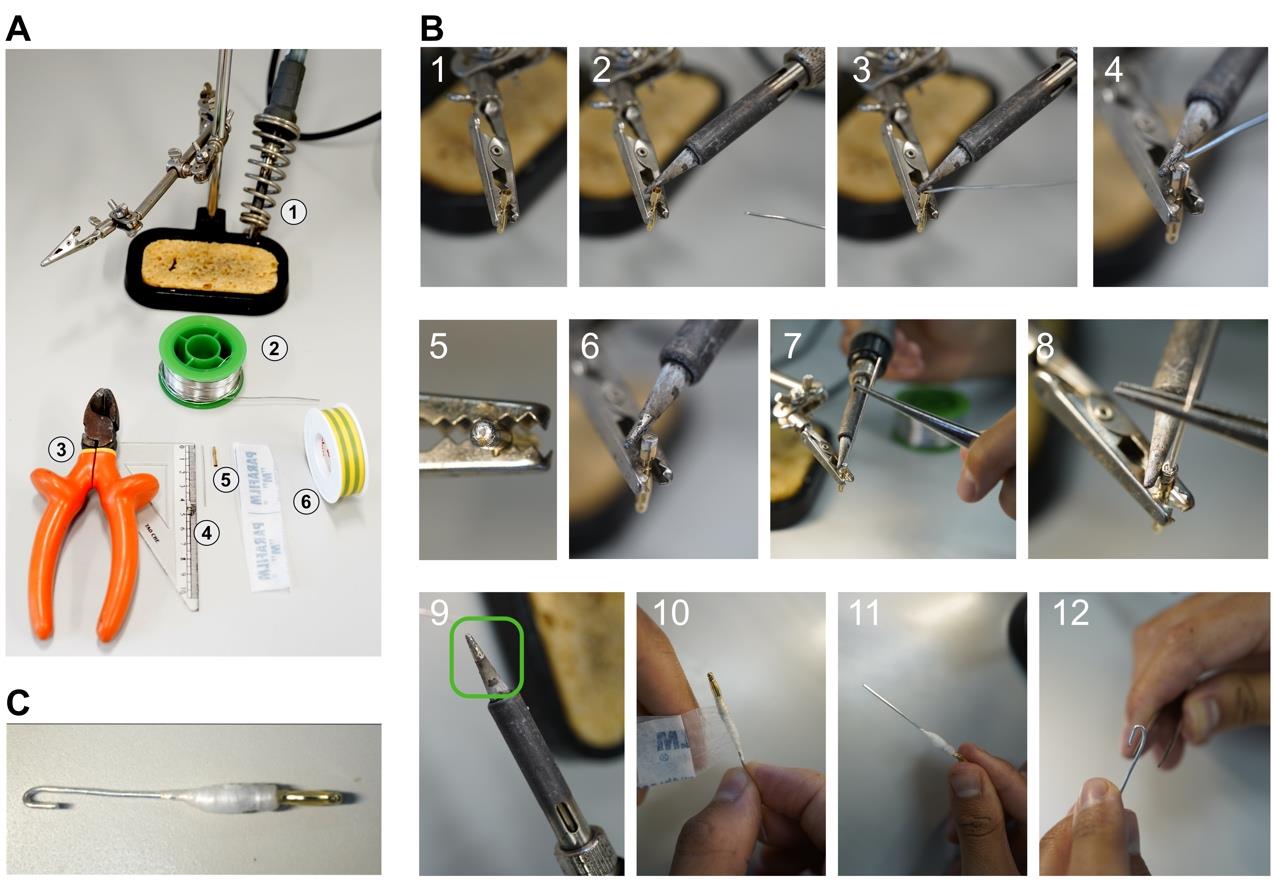
Figure 2. Soldering electrodes for potential recordings. (A) Overview of necessary equipment: (1) soldering iron and holding device, (2) solder, (3) pliers and ruler for cutting the silver wire, (4) silver wire, (5) banana plug, (6) parafilm and insulating tape. (B) Step-by-step soldering instructions: 1. Place the banana plug in the holder. 2. Heat the banana plug with the soldering iron. 3, 4. Fill the empty banana plug with the solder. 5. Close-up of the filled banana plug. 6. Keep the filled banana plug hot to add the silver wire. 7, 8. Add the silver wire. 9. Maintain the soldering iron by cleaning it with the solder, leaving a thin layer of solder on the tip (green rectangle). 10, 11. Wrap the connection of the banana plug and the silver wire with parafilm or insulating tape to isolate it. 12. Bend the tip of the electrode with a forceps into a hook. (C) Finished electrode.
2. Chloridization (at the earliest a day before the recordings)
Note: Chloridize multiple ground and surface electrodes to have enough backups.
a. Dip ~1 cm of the hooked electrode end in freshly prepared 5% NaOCl (see Recipe 2).
b. Allow the reaction to proceed for 30 min.
c. Rinse with 50 mM electrode solution (see Recipe 1) and dry the electrodes with a paper towel.
d. The electrodes can typically be used for ~20 recordings or more.
3. Stripping (Figure 3)
Note: Stripping is performed on used, chloridized electrodes, prior to properly re-chloridizing them for the next experiment.
a. Abrade the used electrodes with emery paper.
b. Dip the tip of the electrodes in 25% ammonium hydroxide and scrape with forceps until lustrous.
Caution: Ammonium hydroxide is hazardous and should only be handled with gloves under the fume hood.
c. Rinse in 50 mM electrode solution. Dry electrodes with a paper towel. Store in dry and dark conditions (see step B2).
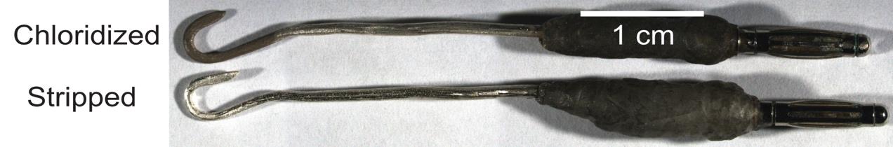
Figure 3. Surface silver chloride electrode. Top: freshly chloridized (see the dark hook); bottom: freshly stripped electrode (see lustrous hook).
C. Setting up the surface potential rig
Note: A Faraday cage helps to reduce electric noise but is not strictly necessary. The ground electrode is placed inside the 1/2 MS solution (see Recipe 4). Avoid direct contact of the electrode with the petiole. Use an electric multimeter to confirm that the setup is properly grounded.
1. Connect the digitizer, amplifier, and head stages as described by the manufacturer.
2. Place the head stages in the micromanipulators on the optical table.
3. Set up the LabScribe software as described by the developer.
4. Stick the bath electrode in a PCR tube filled with bath electrode solution (with 3% LE agar) and physically secure that connection with parafilm (Figure 4A).
5. Cut the tip of that PCR tube with scissors and place it in the 1/2 MS bath solution (Figure 4A).
6. Use enough 1/2 MS media to be able to immerse the electrode (Figure 4A).
7. Separate the wounding and receiving leaves from each other by using pipette tips (Figures 1E and 4B).
8. Place the pot containing the plant to be recorded in a tray with 1/2 MS media (Figure 4C).
9. Place the leaf to be wounded inside the wounding device (Figure 4B).
10. Place electrodes on the petioles of leaves 8 and 13 and connect them via an agar bridge using <20 μL of leaf electrode solution (with 0.8% LE agar) (Figure 4B).
Note: Make sure not to burn the plant with the hot agar. Leave the 0.8% LE agar on the hotplate stirrer to keep it liquid.
11. Ensure that you have a closed, properly grounded circuit (Figure 4C, D; see Troubleshooting).
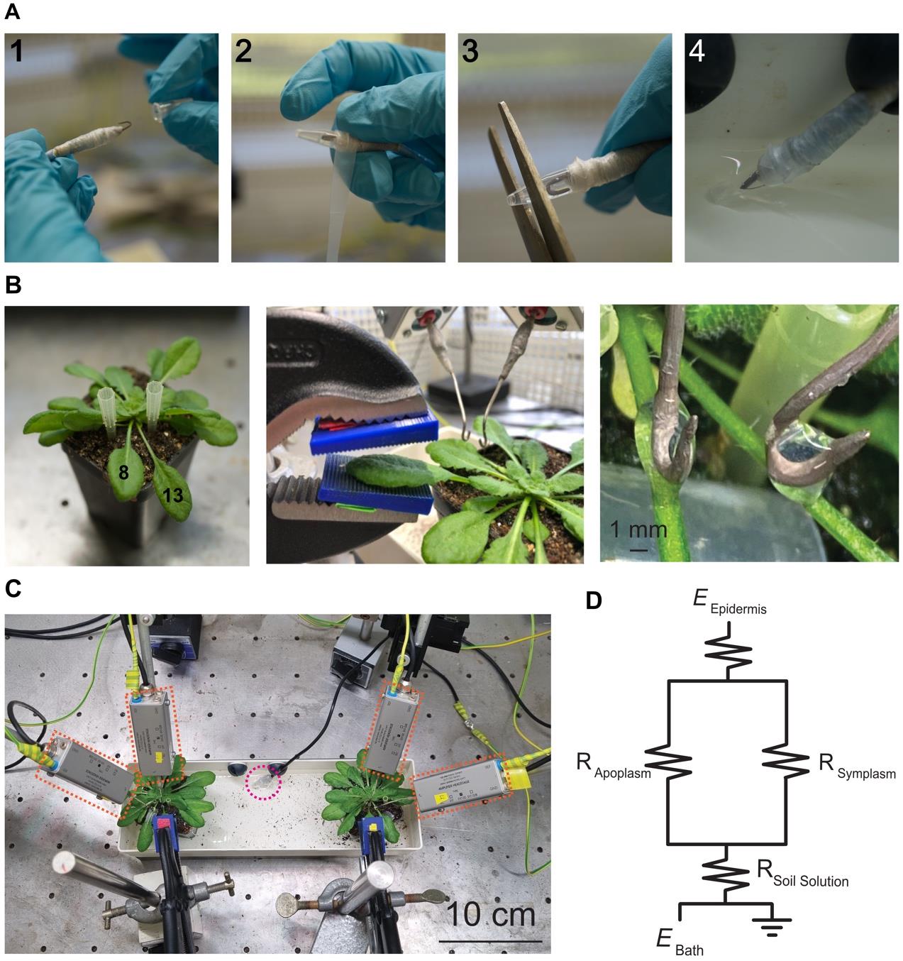
Figure 4. Experimental recording setup and electrode placement. (A) To add the bath electrode to the circuit, first (1) place the electrode into the tube containing the 3% LE agar bath electrode solution, (2) seal the PCR tube on the electrode with parafilm, (3) cut the tip of the tube to have access to the agar, and (4) position the open tube containing the electrode into the bath solution. (B) Separation of leaves 8 and 13 using pipette tips, followed by the placement of leaf 8 inside the clamp. Connect the surface electrode with a 0.8% LE agar bridge. (C) Overview of the setup inside the Faraday cage for simultaneous measurement of two plants. Orange rectangles highlight the head stages for each electrode, and the pink circle marks the bath electrode. All electrodes are grounded to the cage. (D) Schematic circuit (R = resistance, E = electrode).
D. Wounding
Note: Ensure that you can record a stable baseline without drift or noise in LabScribe before starting the actual recording. To properly analyze the data later, mark the end of the wounding (opening of the clamp) with the F1 key in the exported text files. The length of the recording can vary depending on the signal and experiment and is to be adjusted for your specific purposes. Avoid letting the clamps jump open to prevent the movement of the electrodes and noisy recordings. The closing pressure of the clamp can be adjusted with the screw in the back. Adjust it with the 3D-printed grids in place to a pressure in which the leaf is totally flaccid and translucent but not severed after wounding (Figure 5D). Use similar pressure for all plants.
1. Ensure that approximately 2/3 of the leaf blade area is placed inside the clamp holding the 3D-printed grids (Figures 4B, 5A, 5D).
2. Before wounding, record a baseline for 90 s.
3. Close the clamp completely for 5 s (Figure 5B).
4. Carefully open the clamp.
5. Record for at least 10 min in total (Figure 5C).
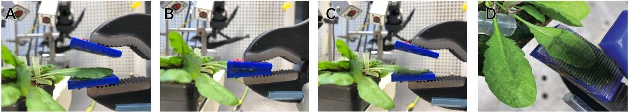
Figure 5. Wounding process during the recording. (A) Placement of the leaf between the clamp. (B) Closed clamp on the leaf; hold for 5 s in this position. (C) Opening of the clamp. (D) Leaf post wounding.
Data analysis
Note: Consistent annotation of the data set is crucial for the proper execution of the script.
The slow wave potential (SWP) typically consists of at least three phases: an initial hyperpolarization, a depolarization, and a repolarization often followed by a secondary hyperpolarization. Each phase is defined by multiple parameters (Figure 6). These parameters can be analyzed from a single trace. To automate the determination of six different parameters, we developed the R script SWPanalyzer.Rmd, which is available on GitHub here.
The script was designed to handle data obtained using the LabScribe and LabView NI software. It can analyze recordings from up to two simultaneously measured plants, with one electrode on the wounded leaf and another on a non-wounded leaf.
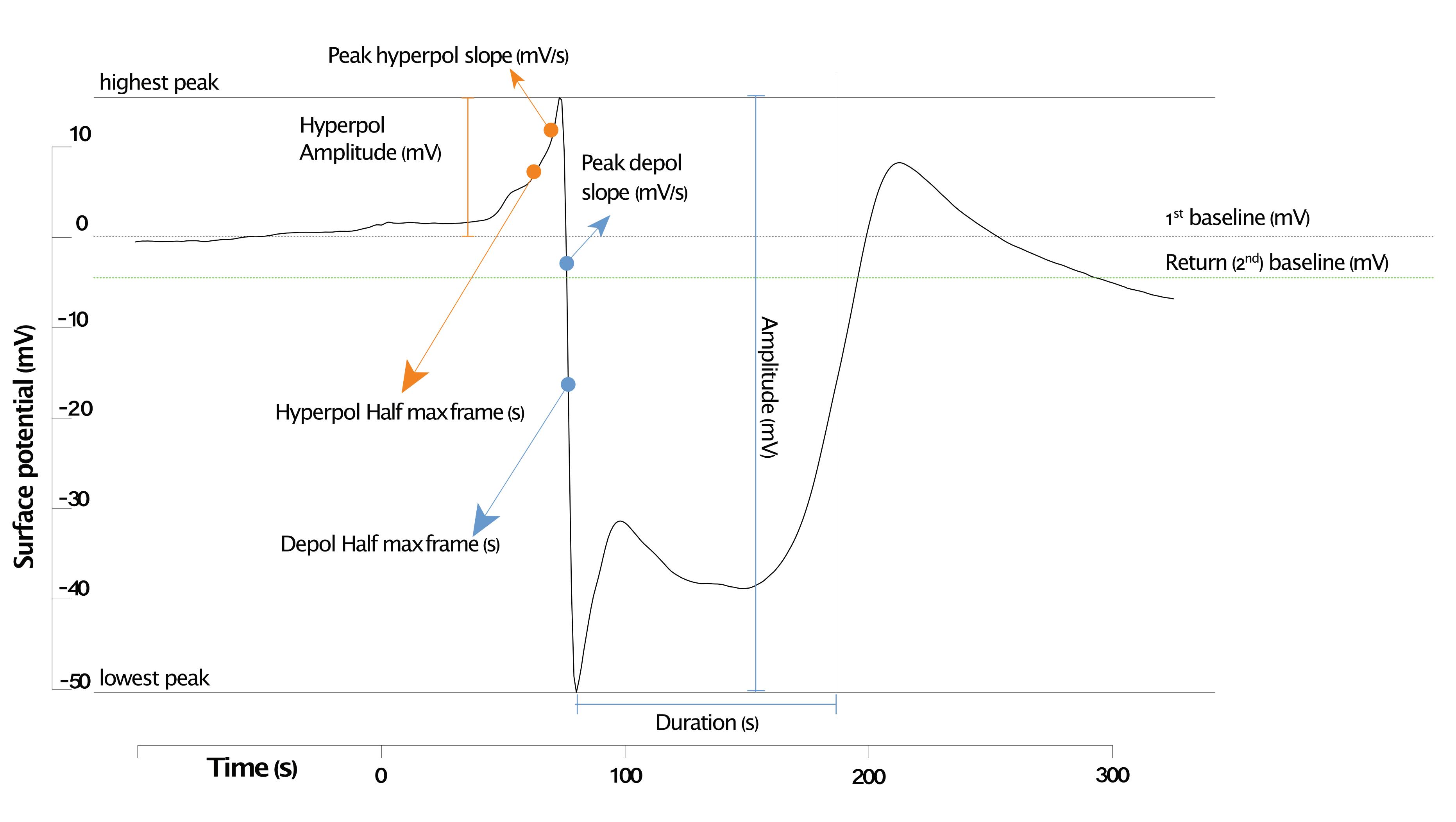
Figure 6. Exemplary Col-0 surface potential curve of leaf 13 with all parameters identified using the script. The quantified parameters of the first hyperpolarization are highlighted in orange; the parameters of the depolarization are in blue. The first baseline (dashed grey line) is the baseline before wounding, and the second is the baseline (dashed green line) after repolarization.
1. Annotate files:
Label the electrode recording on leaf 8 with all relevant experimental details (e.g., genotype, leaf number, and treatments). Organize this information according to the format specified in the script description.
2. Export .txt files for analysis:
Once the recording is saved, export it to a .txt file by selecting File > Export. In the window that appears, check the box for “Include time of day.” The sampling rate can be set to either 10 or 100 Hz, with 100 Hz being sufficient for data visualization. Gather all files in a single folder named after the recording date in the format yymmdd. The specific name of each file is irrelevant to the script. The folder(s) containing recordings from different days will serve as the initial input for the script.
3. How to use the script:
To run the script, create a new project in R Studio by selecting File > New Project. In the window that opens, choose New Directory > New Project. Enter a name for the folder (e.g., “home”) and select a path where it will be created. This home folder will contain the project file (home.Rproj). Place all yymmdd folders containing the exported data into this home folder. Open the script by selecting File > Open and choosing the downloaded SWPanalyzer.Rmd file. Read the description and follow the instructions provided in the script.
The first four sections of the script cover the minimum analysis required. After running these sections successfully, the following output files will be generated in the home folder:
• A genotype.csv file for each genotype measured, containing all recorded traces.
• A genotypeSummary.csv file with the calculated parameters for all leaves of all plants.
• A mean-genotype-Lxx.pdf file for each genotype, featuring a mean trace with an overlaid standard error of the mean (±SEM) of all traces (Figure 7A). The traces included in this mean plot can be manually selected in Section 5.
• A genotype-yymmdd folder containing plots of each leaf of each plant, with overlays of the calculated parameters and a graphic visualization of the data as a violin plot (Figure 7B), comparing results between genotypes (yymmdd-parameter.pdf).
After running the script, visually inspect the quantified parameters by checking the #.Lxx.pdf images generated for each trace. If a parameter is wrongly quantified, you can trace it back to the genotypeSummay.csv by the date, the #, and the leaf, and exclude it from further statistical analysis.
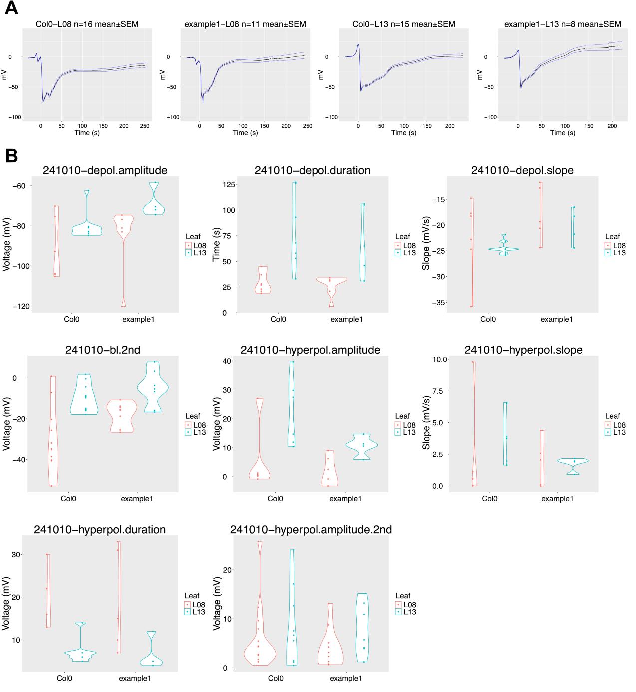
Figure 7. SWPanalyzer.Rmd output of the analyzed exemplary dataset from recordings of Col-0 and mutant (example 1) plants. (A) Mean traces ± SEM error bands of all analyzed traces for leaves (L) 8 and 13. (B) Violin plots for each parameter. Depol = depolarization, bl= baseline. Each dot represents one recording.
Validation of protocol
This protocol is a robust and reproducible way to study SWPs of plant surfaces. The number of replicates needed is typically≥10 in order to apply statistical tests (e.g., to compare genotypes). Col-0 plants were employed for surface potential recordings (see Figures 1, 2, 4, and 5). The data obtained was analyzed using the SWPanalyzer.Rmd (see Data analysis). The raw data can be found here. Parts of this protocol have been used in [10].
General notes and troubleshooting
General notes
1. Although this protocol uses the Arabidopsis thaliana Col-0 ecotype, other ecotypes may be used. However, differences in rosette morphology could affect petiole accessibility for electrode placement.
2. Prior to the measurement, plants should be acclimatized to the new conditions.
3. The raw data, analysis, R script, and 3D design can be found under the following link: https://github.com/jucbca/SWP-data_analysis
Troubleshooting
Recording:
Problem: You are unable to record any changes in electric potentials.
Solutions:
1. If you do not detect a signal in the wounded leaf:
a. Use a lighter to burn the leaf from the bottom. This method is the most reliable trigger of SWPs and serves as a positive control for your setup.
b. Check with a multimeter to see if all connections are properly grounded to the same ground.
c. By visual inspection, ensure the ground electrode is still chloridized. If not, exchange it.
d. Verify that the surface potential electrode is properly connected via an agar bridge. If necessary, exchange the electrodes.
2. If you are able to record a signal in the wounded leaf but not in the distal leaf:
a. Verify that the leaves were counted correctly.
Problem: You are unable to offset the voltage in the amplifier to 0. It is out of range, keeps drifting, or presents high noise.
Solutions:
1. If the problem occurs for all electrodes:
a. Increase the volume of 1/2 MS in the pot container.
b. Ensure the ground electrode is still chloridized. If not, exchange it.
2. If the problem occurs for only one electrode:
a. Ensure the recording electrode is still chloridized. If not, exchange it.
b. Verify that the surface potential electrode is properly connected via an agar bridge. If necessary, exchange the electrodes.
Data analysis:
Section 1: Ensure you run this section every time the project is opened.
Section 2:
Problem: Different folders are created for the same genotype.
Solution: Ensure the spelling of the genotype is consistent across all electrode labels in the .txt files. Variations in spaces, capital letters, or dashes will cause the script to identify them as different genotypes (e.g., Col0, col0, Col 0, Col-0).
Section 3:
Problem: A trace generates aberrant parameters, causing Chunk 3.2 to stop running.
Solution: Re-run Chunk 3.2 and remove the problematic trace. This trace cannot be analyzed due to poor recording quality.
Acknowledgments
This work was funded by the Deutsche Forschungsgemeinschaft (DFG, German Research Foundation) under Germany’s Excellence Strategy – EXC-2048/1 – project ID 390686111 (CEPLAS) and under project ID 267205415-CRC 1208. We thank Dr. Marriah Green for the critical reading of the manuscript and Waldemar Seidel for help in the rig setup. This protocol was used in [10].
Competing interests
The authors declare no competing interests.
References
- Mousavi, S. A. R., Nguyen, C. T., Farmer, E. E. and Kellenberger, S. (2014). Measuring surface potential changes on leaves. Nat Protoc. 9(8): 1997–2004. https://doi.org/10.1038/nprot.2014.136
- Burdon-Sanderson, J. S. (1873) I. Note on the Electrical Phenomena Which Accompany Irritation of the Leaf of Dionæa Muscipula. Proc R Soc Lond. 21: 495–496. https://doi.org/10.1098/RSPL.1872.0092.
- Umrath, K. (1930). Untersuchungen über Plasma und Plasmaströmung an Characeen. Protoplasma. 9(1): 576–597. https://doi.org/10.1007/bf01943373
- Schroeder, J. I., Hedrich, R. and Fernandez, J. M. (1984). Potassium-selective single channels in guard cell protoplasts of Vicia faba. Nature. 312(5992): 361–362. https://doi.org/10.1038/312361a0
- Lautner, S., Grams, T. E. E., Matyssek, R. and Fromm, J. (2005). Characteristics of Electrical Signals in Poplar and Responses in Photosynthesis. Plant Physiol. 138(4): 2200–2209. https://doi.org/10.1104/pp.105.064196
- Fromm, J. and Lautner, S. (2006). Electrical signals and their physiological significance in plants. Plant Cell Environ. 30(3): 249–257. https://doi.org/10.1111/j.1365-3040.2006.01614.x
- Vodeneev, V., Akinchits, E. and Sukhov, V. (2015). Variation potential in higher plants: Mechanisms of generation and propagation. Plant Signal Behav. 10(9): e1057365. https://doi.org/10.1080/15592324.2015.1057365
- Doran, L. (2021) Sterilizing the Surface of Seeds by Chlorine Gas V.1. Protocols.Io. https://doi.org/10.17504/protocols.io.bx8rprv6
- Farmer, E., Farmer, E., Mousavi, S. and Lenglet, A. (2013). Leaf numbering for experiments on long distance signalling in Arabidopsis. Protocol Exchange. e071. https://doi.org/10.1038/protex.2013.071
- Moe-Lange, J., Gappel, N. M., Machado, M., Wudick, M. M., Sies, C. S. A., Schott-Verdugo, S. N., Bonus, M., Mishra, S., Hartwig, T., Bezrutczyk, M., et al. (2021). Interdependence of a mechanosensitive anion channel and glutamate receptors in distal wound signaling. Sci Adv. 7(37): eabg4298. https://doi.org/10.1126/sciadv.abg4298
Article Information
Publication history
Received: Nov 8, 2024
Accepted: Feb 20, 2025
Available online: Mar 12, 2025
Published: Apr 5, 2025
Copyright
© 2025 The Author(s); This is an open access article under the CC BY-NC license (https://creativecommons.org/licenses/by-nc/4.0/).
How to cite
Readers should cite both the Bio-protocol article and the original research article where this protocol was used:
- Atanjaoui, F., Kleist, T. J., Barbosa-Caro, J. C. and Wudick, M. M. (2025). A Detailed Guide to Recording and Analyzing Arabidopsis thaliana Leaf Surface Potential Dynamics Elicited by Mechanical Wounding. Bio-protocol 15(7): e5252. DOI: 10.21769/BioProtoc.5252.
- Moe-Lange, J., Gappel, N. M., Machado, M., Wudick, M. M., Sies, C. S. A., Schott-Verdugo, S. N., Bonus, M., Mishra, S., Hartwig, T., Bezrutczyk, M., et al. (2021). Interdependence of a mechanosensitive anion channel and glutamate receptors in distal wound signaling. Sci Adv. 7(37): eabg4298. https://doi.org/10.1126/sciadv.abg4298
Category
Plant Science > Plant cell biology > Intercellular communication
Cell Biology > Cell signaling > Stress response
Do you have any questions about this protocol?
Post your question to gather feedback from the community. We will also invite the authors of this article to respond.