- Protocols

- Articles and Issues
- For Authors
- About
- Become a Reviewer

Time-Lapse Super-Resolution Imaging and Optical Manipulation of Growth Cones in Elongating Axons and Migrating Neurons

(*contributed equally to this work) Published: Vol 15, Iss 6, Mar 20, 2025 DOI: 10.21769/BioProtoc.5251 Views: 2184
Reviewed by: Anthony FlamierAnonymous reviewer(s)
Original research article
The authors used this protocol in:

Mar 2024
Advertisement


Protocol Collections
Comprehensive collections of detailed, peer-reviewed protocols focusing on specific topics


Abstract
The growth cone is a highly motile tip structure that guides axonal elongation and directionality in differentiating neurons. Migrating immature neurons also exhibit a growth cone–like structure (GCLS) at the tip of the leading process. However, it remains unknown whether the GCLS in migrating immature neurons shares the morphological and molecular features of axonal growth cones and can thus be considered equivalent to them. Here, we describe a detailed method for time-lapse imaging and optical manipulation of growth cones using a super-resolution laser-scanning microscope. To observe growth cones in elongating axons and migrating neurons, embryonic cortical neurons and neonatal ventricular–subventricular zone (V-SVZ)-derived neurons, respectively, were transfected with plasmids encoding fluorescent protein–conjugated cytoskeletal probes and three-dimensionally cultured in Matrigel, which mimics the in vivo background. At 2–5 days in vitro, the morphology and dynamics of these growth cones and their associated cytoskeletal molecules were assessed by time-lapse super-resolution imaging. The use of photoswitchable cytoskeletal inhibitors, which can be reversibly and precisely controlled by laser illumination at two different wavelengths, revealed the spatiotemporal regulatory machinery and functional significance of growth cones in neuronal migration. Furthermore, machine learning–based methods enabled us to automatically segment growth cone morphology from elongating axons and the leading process. This protocol provides a cutting-edge methodology for studying the growth cone in developmental and regenerative neuroscience, being adaptable for various cell biology and imaging applications.
Key features
• Three-dimensional primary culture of migrating and differentiating neurons in Matrigel.
• Visualization of fine morphology and dynamics of growth cones using super-resolution imaging.
• Optical manipulation of cytoskeletal molecules in growth cones using photoswitchable inhibitors.
• Machine learning–based extraction of growth cone morphology.
Keywords: Growth coneGraphical overview

Background
The growth cone is a highly motile subcellular structure observed at the tip of elongating axons and involved in the determination of their directionality [1]. Since its first description by Santiago Ramón y Cajal in 1890 [2], the morphology, dynamics, and regulatory mechanisms of the axonal growth cone have been intensively studied. The growth cone consists of central and peripheral domains that are enriched with microtubule networks and filamentous actin (F-actin), respectively [3]. During the elongation process of the growth cone, F-actin polymerization first occurs at its peripheral domain to form specialized membrane protrusions such as filopodia and lamellipodia, followed by microtubule polymerization and subsequent growth cone extension [3]. These cytoskeletal dynamics in the growth cone are affected by various axonal guidance cues and extracellular matrix molecules, which ensure the appropriate projection of elongating axons [1]. Previous studies suggested that inhibition of F-actin and microtubules in the growth cone disrupts its formation and axonal elongation, suggesting that cytoskeletal dynamics in the growth cone is a central regulator for axonal elongation. Thus, time-lapse imaging of the growth cone and its associated cytoskeleton at a super-resolution level could be a potent methodology for a better understanding of its regulatory mechanisms and the establishment of novel strategies for neuronal regeneration following injury in the nervous system.
Newborn neurons are generated from neural stem cells in the embryonic and postnatal stages and show immature migratory morphology with a long leading process and a short trailing process [4]. During the migration process, these new neurons form a growth cone–like structure (GCLS) at the tip of their leading process and extend it, followed by somal translocation [5]. New neurons continue to migrate toward their final destinations by repeating these steps, which implies that the GCLS plays a central role in neuronal migration. Recent studies showed that cytoskeletal molecules in the GCLS are involved in the generation of the traction forces for efficient migration of cerebellar granule cells [6]. However, it remains unknown whether the GCLS in migrating neurons is morphologically and molecularly similar to growth cones in elongating axons.
We have recently performed comprehensive comparison analyses between growth cones in elongating axons and GCLS in migrating neurons [7]. By performing time-lapse super-resolution imaging of F-actin and microtubule dynamics, we revealed that the GCLS on the leading process of migrating neurons is morphologically and dynamically analogous to the axonal growth cone, suggesting that migrating neurons also possess a growth cone. In addition, axonal growth cone molecules were also concentrated in the leading process growth cone of migrating neurons, indicating common molecular features in axonal and leading process growth cones. Furthermore, spatiotemporal optical manipulation of cytoskeletal molecules using photoswitchable inhibitors revealed the regulatory mechanism and functional significance of the growth cone in neuronal migration. Here, we describe detailed protocols for time-lapse super-resolution imaging and optical manipulation of cytoskeletal molecules in growth cones [7]. This methodology is a basis for the fields of growth cone research in developmental and regenerative neuroscience and is also widely applicable to various types of cells in cell biology and imaging studies.
Materials and reagents
Biological materials
1. Embryonic day 15.5–16.5 (E15.5–16.5) C57BL/6J or Institute of Cancer Research (ICR) mice (Japan SLC)
2. Postnatal day 0–1 (P0–1) C57BL/6J or Institute of Cancer Research (ICR) mice (Japan SLC)
Reagents
1. Leibovitz’s L15 medium (Gibco, catalog number: 11415-064)
2. DMEM high glucose (Sigma-Aldrich, catalog number: D5796)
3. Neurobasal medium (Gibco, catalog number: 21103)
4. HBSS, no calcium, no magnesium (Thermo Fischer Scientific, catalog number: 14170112)
5. Penicillin-streptomycin (penicillin, 10,000 units/mL; streptomycin, 10,000 μg/mL) (Gibco, catalog number: 15140-122)
6. GlutaMAX (Thermo Fisher Scientific, catalog number: 35050061)
7. NeuroBrew-21 (MACS Miltenyi Biotec, catalog number: 130-093-566)
8. DNase I (1 mg/mL stock solution) (Roche, catalog number: 10-104-159-001)
9. 0.25% (w/v) trypsin 1 mmol/L EDTA·4Na solution with phenol red, 500 mL (Wako, catalog number: 201-16945)
10. RPMI-1640 medium (Wako, catalog number: 189-02145)
11. BD Matrigel matrix, 10 mL (BD Biosciences, catalog number: 354234)
12. Fetal bovine serum (FBS) (Gibco, catalog number: 10437)
13. HEPES (Sigma-Aldrich, catalog number: H0887)
14. Trypsin inhibitor from soybean (Wako, catalog number: 206-20121)
15. Bovine serum albumin (BSA) (Sigma-Aldrich, catalog number: A3059)
16. Magnesium sulfate heptahydrate (Wako, catalog number: 131-00405)
17. AmaxaTM Mouse Neuron NucleofectorTM kit (Lonza, catalog number: VPG-1001)
18. AmaxaTM P3 Primary Cell 4D-NucleofectorTM X kit L (Lonza, catalog number: V4XP-3024)
19. KE-106 (Shin-Etsu Silicone) [8]
20. CAT-RG (Shin-Etsu Silicone) [8]
21. India ink [8]
22. Opto-Latrunculin (Opto-Lat) [9]
23. Phenyl-neo-Optojasp (PnOJ) [10]
24. Photostatin-1 (PST-1) [11]
25. Dimethylsulfoxide (DMSO) (Sigma-Aldrich, catalog number: D8418-100 mL)
26. AlexaFluor 647-conjugated bovine serum albumin (2 mM) (Invitrogen, catalog number: A34785)
27. Recombinant Neurocan (Ncan) (R&D Systems, catalog number: 5800-NC-050)
28. Recombinant Syndecan-2 (Sdc2) (R&D Systems, catalog number: 6585-SD-050)
29. pCAGGS-Venus-CAAX (4.0 μg/mL stock solution) [7]
30. pCAGGS-tdTomato-CAAX (4.0 μg/mL stock solution) [7]
31. pCAGGS-DsRed-miR-lacZ (4.0 μg/mL stock solution) [7]
32. pAcGFP1-actin (GFP-actin), 4.0 μg/mL stock solution) (Clontech, catalog number: Z2453N)
33. pcDNA3.1-EB3-EGFP (4.0 μg/mL stock solution) [kind gift from K. Kaibuchi (Fujita Health University, Japan)] [12]
34. pCS2-EGFP-UtrCH (4.0 μg/mL stock solution) [kind gift from W. Bement (University of Wisconsin-Madison) and D. J. Solecki (St. Jude Children’s Research Hospital)] [13]
35. Paraformaldehyde (PFA) (Wako, catalog number: 168-20955)
36. Sodium dihydrogen phosphate dihydrate (Kanto, catalog number: 37239-00)
37. Disodium hydrogen phosphate dodecahydrate (Wako, catalog number: 198-02834)
38. Sodium chloride (Wako, catalog number: 195-01663)
39. Potassium chloride (Sigma-Aldrich, catalog number: P9541)
40. Potassium dihydrogen phosphate (Wako, catalog number: 169-04245)
41. Normal donkey serum (Sigma-Aldrich, catalog number: S30-100ML)
42. Triton X-100 (Sigma-Aldrich, catalog number: X100)
43. AlexaFluor 488-conjugated phalloidin (1:100) (Invitrogen, catalog number: A12379)
44. Anti-tyrosinated tubulin antibody (1:200) (Sigma, catalog number: MAB1864-I)
45. Anti-acetylated tubulin antibody (1:200) (Sigma, catalog number: T6793)
46. AlexaFluor 594-conjugated donkey anti-rat IgG (H+L) highly cross-absorbed secondary antibody (1:1,000) (Thermo Fisher Scientific, catalog number: A-21209)
47. AlexaFluor 647-conjugated donkey anti-mouse IgG (H+L) highly cross-absorbed secondary antibody (1:1,000) (Thermo Fisher Scientific, catalog number: A-31571)
48. Hoechst 33342 (10 mg/mL stock solution; 1:5,000) (Invitrogen, catalog number: H3570)
49. VECTASHIELD vibrance antifade mounting medium (Vector Laboratories, catalog number: H-1700)
Solutions
1. DMEM culture medium (see Recipes)
2. Dissociation buffer (see Recipes)
3. 75% Matrigel/L15 medium (see Recipes)
4. Neurobasal final medium (see Recipes)
5. 60% Matrigel/Ncan/L15 medium (see Recipes)
6. DNase I solution (see Recipes)
7. 10% FBS/L15 medium (see Recipes)
8. Sdc2/BSA-alexa647 solution (see Recipes)
9. 4% PFA in 0.1 M PB (see Recipes)
10. 1× PBS (see Recipes)
11. Blocking solution (see Recipes)
12. Silicone solution (see Recipes)
Recipes
1. DMEM culture medium
| Reagent | Final concentration | Quantity or Volume |
|---|---|---|
| DMEM high glucose | - | 10 mL |
| FBS | - | 1 mL |
| GlutaMAX (200 mM) | 2 mM | 100 μL |
| NeuroBrew-21 | 2% | 200 μL |
| Penicillin-streptomycin | 50 U/mL | 100 μL |
2. Dissociation buffer
| Reagent | Final concentration | Quantity or Volume |
|---|---|---|
| BSA | 3 mg/mL | 150 mg |
| Magnesium sulfate heptahydrate | 12 mM | 60 mg |
| DNase I | 0.025% | 12.5 mg |
| Trypsin inhibitor from soybean | 0.4 mg/mL | 20 mg |
| 1 M HEPES | 10 mM | 500 μL |
| HBSS | Fill up to 50 mL |
3. 75% Matrigel/L15 medium
| Reagent | Final concentration | Quantity or Volume |
|---|---|---|
| L15 medium | - | 25 μL |
| Matrigel | 75% | 75 μL |
4. Neurobasal final medium
| Reagent | Final concentration | Quantity or Volume |
|---|---|---|
| Neurobasal medium | - | 10 mL |
| GlutaMAX (200 mM) | 2 mM | 100 μL |
| NeuroBrew-21 | 2% | 200 μL |
| Penicillin-streptomycin | 50 U/mL | 100 μL |
5. 60% Matrigel/Ncan/L15 medium
| Reagent | Final concentration | Quantity or Volume |
|---|---|---|
| L15 medium | - | 30 μL |
| Ncan (300 μg/mL) | 30 μg/mL | 10 μL |
| Matrigel | 60% | 60 μL |
6. DNase I solution
| Reagent | Final concentration | Quantity or Volume |
|---|---|---|
| L15 medium | - | 10 mL |
| DNase I (1 mg/mL stock solution) | 40 μg/mL | 400 μL |
7. 10% FBS/L15 medium
| Reagent | Final concentration | Quantity or Volume |
|---|---|---|
| L15 medium | - | 9 mL |
| FBS | 10% | 1 mL |
8. Sdc2/BSA-alexa647 solution
| Reagent | Final concentration | Quantity or Volume |
|---|---|---|
| Sdc2 (200 μg/mL) | 2 mM (28 μg/mL) | 28 μL |
| AlexaFluor 647-conjugated bovine serum albumin (2 mM) | 5 μM | 0.5 μL |
| L15 medium | - | 172 μL |
9. 4% PFA in 0.1 M PB
| Reagent | Final concentration | Quantity or Volume |
|---|---|---|
| PFA | 4% | 4 g |
| Sodium dihydrogen phosphate dihydrate (31.2 g/L stock solution) | 0.1 M | 10 mL |
| Disodium hydrogen phosphate dodecahydrate (71.6 g/L stock solution) | 0.1 M | 40 mL |
| Distilled water | - | Fill up to 100 mL |
10. 1× PBS
| Reagent | Final concentration | Quantity or Volume |
|---|---|---|
| Sodium chloride | - | 40 g |
| Disodium hydrogen phosphate dodecahydrate | - | 18.15 g |
| Potassium chloride | - | 1 g |
| Potassium dihydrogen phosphate | - | 1.2 g |
| H2O | - | Fill up to 5 L |
11. Blocking solution
| Reagent | Final concentration | Quantity or Volume |
|---|---|---|
| Normal donkey serum | 10% | 1 mL |
| PBS | - | 9 mL |
| Triton X-100 (20% stock solution) | 0.2% | 100 μL |
12. Silicone solution [8]
| Reagent | Final concentration | Quantity or Volume |
|---|---|---|
| KE-106 | - | 23 mL |
| CAT-RG | - | 2.3 mL |
| India ink | - | 0.6 mL |
Add the mixed silicone solution to a 35 mm dish and polymerize it by incubation at 60 °C for 3 h in an incubator to make a silicone-based 35 mm dissection Petri dish.
Laboratory supplies
1. 70 μm cell strainer (Corning, catalog number: 352350)
2. 35 mm multi-well glass-bottom dish (Matsunami, catalog number: D141400)
3. 35 mm tissue culture dish (Corning, catalog number: 353001)
4. 100 mm tissue culture dish (BD Falcon, catalog number: 353003)
5. 50 mL centrifuge tube (Thermo Fischer Scientific, catalog number: 339652)
6. 1.5 mL microtube (BIO-BIK, catalog number: CF-0150)
7. 0.6 mL microtube (QSP, catalog number: 502-PLN-Q)
Equipment
1. ZEISS Stemi 508 (Carl Zeiss, catalog number: 495009-0008-000)
2. Microscopic scissors (Karl Hammacher GmbH, model: HSB014-11)
3. Forceps (Natsume Seisakusyo Co., Ltd., model: NAPOX A-1)
4. Ultrafine forceps (Dumont, model: DU-5/45)
5. Ophthalmic knife (MANI, model: MST15)
6. P1000 micropipette (Nichiryo, catalog number: NPX-1000)
7. P200 micropipette (Nichiryo, catalog number: NPX-200)
8. P20 micropipette (Nichiryo, catalog number: NPX-20)
9. P2 micropipette (GILSON, catalog number: F144801)
10. Amaxa NucleofectorTM II (Lonza, catalog number: AAB-1001)
11. Amaxa 4D-Nucleofector X unit (Lonza, catalog number: AAF-1003X)
12. Amaxa 4D-Nucleofector core unit (Lonza, catalog number: AAF-1003B)
13. Centrifuge (TOMY, model: PMC-060)
14. Matrix 2C (for stripe assay, 40 μm parallel, Martin Bastmeyer) (Zoologisches Institut Abteilung für Zell- und Neurobiologie) [14]
15. Super-resolution laser-scanning microscope system (Carl Zeiss, model: LSM880 with Airyscan FAST)
16. Laser diode 405 nm CW (Carl Zeiss, catalog number: 000000-2031-918)
17. Laser line 561 (Carl Zeiss, catalog number: 000000-1410-117)
18. Laser Argon Multiline 25 mW (Carl Zeiss, catalog number: 000000-2086-081)
19. Laser Rack LSM880 incl. 633 nm Laser (Carl Zeiss, catalog number: 000000-2085-478)
20. Spectral detector 32 channels GaAsP PMT plus 2 channels MA-PMT (Carl Zeiss, catalog number: 000000-2179-906)
21. Airyscan module for LSM880, with super-resolution and virtual pinhole function (Carl Zeiss, catalog number: 000000-2058-0580)
22. 40× water-immersion objective lens (Carl Zeiss, model: NA1.2)
23. 63× oil-immersion objective lens (Carl Zeiss, model: NA1.4)
24. Immersol W (2010) (Carl Zeiss, catalog number: 444969-0000-000)
25. Immersol 518F/30 °C (Carl Zeiss, catalog number: 444970-9000-000)
26. Stage-top incubation chamber (Tokai Hit Co., Ltd., catalog number: INUG2-WSKM)
27. CO2 gas tank
28. CO2 incubator (PHCbi, model: MCO-170AICUV)
29. Incubator (EYELA, model: NDS-500)
30. Beads bath (Lab Armor Bead Bath 6L, model: 74300-706)
31. Benchtop centrifuge (TOMY Digital Biology, model: Multi Spin 00-NCF)
Software and datasets
1. ZEN (Carl Zeiss)
2. Trainable Weka Segmentation plugin in FIJI (https://fiji.sc) [15]
3. EZR (https://www.softpedia.com/get/Science-CAD/EZR.shtml) [16]
Procedure
A. Primary culture of differentiating cortical neurons in Matrigel
Primary cultured cortical neurons were prepared from E15.5–16.5 mouse brains and served as differentiating neurons to examine axonal growth cones in the following experimental sections E–J.
Part 1. Brain tissue dissection and dissociation
1. Euthanize a pregnant mouse, collect E15.5–16.5 embryos in a 100 mm tissue culture dish with ice-cold L15 medium, and decapitate them. Use two embryos per experimental group.
2. Under the microscope, use two pairs of ultrafine forceps to tear the scalp and skull along the midline of the head and open the skull. Lift the brain using forceps and keep the brain in fresh ice-cold L15 medium in a 35 mm tissue culture dish.
Critical: The dissection procedure should be performed within 30 min.
3. Divide the brain into two hemispheres and remove the hindbrain, hippocampus, and olfactory bulbs with forceps in a silicone-based 35 mm dissection Petri dish. Peel off meninges from tissues using forceps without damaging the cortex [17].
4. Transfer the cortices from four embryos to a 1.5 mL Eppendorf tube, mince the tissue into two or three pieces with forceps, and add 200 μL of ice-cold L15 medium to allow the tissue to sediment to the bottom of the tube in the following step.
5. Briefly spin down the tissue and remove the L15 medium from the tube. Add 200 μL of ice-cold 0.05% Trypsin-EDTA (pre-dilute 0.25% Trypsin-EDTA solution with L15) and incubate the tissue for 25 min at 37 °C. Tap the tube every 10 min to mix the tissue well.
6. Add 200 μL of room temperature (RT) FBS to the tissue and tap the tube. Spin down the tissue with a benchtop centrifuge for 30 s (max ca. 2,500× g). Remove the supernatant.
7. Add 200 μL of dissociation buffer to the tissue and titrate the suspension five times with a P1000 and 10 times with a P200 pipette until the suspension is homogeneous.
8. Centrifuge the tube at 80× g for 5 min. Remove the supernatant from the tube.
Proceed to Part 2 for the primary culture of differentiating cortical neurons in Matrigel or to Section B for transfection of cortical neurons.
Part 2. Primary culture of cortical neurons
9. Carefully add 500 μL of ice-cold L15 medium to the tube. Flush the medium using a P200 pipette to the adhering part of the cell pellet and carefully lift the pellet from the tube surface.
10. Transfer the cell pellet to a 35 mm dissection Petri dish with pre-chilled L15 medium. Prepare 0.5–1 mm3 cell aggregate cubes from the cell pellet using an ophthalmic knife and ultrafine forceps.
11. Place a 5 μL 75% Matrigel/L15 drop on a glass-bottom dish and keep the dish on ice.
12. Prepare a fresh 35 mm tissue culture dish with a 10 μL 75%/L15 Matrigel drop. Transfer a cell aggregate (from step A10) to the Matrigel drop using a P20 pipette.
Critical: Do not transfer more than 7 μL of L15 medium with cell aggregate to the Matrigel drop, because a Matrigel concentration lower than 50% will result in the failure of gelation (step A14).
13. Suck the cell aggregate together with 10 μL of Matrigel and place it on a 5 μL Matrigel drop on the glass-bottom dish (step A11). Incubate the glass-bottom dish on ice for 1 min to let the pellet adhere to the bottom of the dish.
14. Incubate the glass-bottom dish for 25 min at 37 °C in the presence of 5% CO2 for Matrigel gelation.
15. Carefully add 200 μL of prewarmed DMEM culture medium and culture the cell aggregates for 3 days at 37 °C in the presence of 5% CO2.
B. Nucleofection of primary cortical neurons
Note: Use the AmaxaTM Mouse Neuron NucleofectorTM kit for the following procedures.
1. Prepare mouse neuron Nucleofector® solution (from the Mouse Neuron Nucleofector kit; see manufacturer’s instructions).
2. Add 200 μL of the Nucleofector solution at RT to the cell pellet (step A8) and suspend the cells gently.
3. Mix 100 μL of cell suspension with plasmid(s) in a fresh Eppendorf tube.
Critical: Excess of plasmid DNA can contribute to cellular toxicity. The total amount of plasmids should not exceed 2.0 μg per tube. The amount of each plasmid DNA used in the study was 0.2–1.8 μg per tube, depending on the expression level of the fluorescent proteins.
4. Transfer the cell suspension into a supplied cuvette without air bubbles using a supplied plastic pipette.
5. Set the cuvette into the cuvette holder of an Amaxa NucleofectorTM II and run the program O-005.
6. Take out the cuvette, add 300 μL of pre-equilibrated RPMI-1640 medium to the cuvette, and gently transfer it to a fresh tube.
7. Incubate the cell suspension for 15 min at 37 °C in the presence of 5% CO2 (recovery step).
8. Spin the tube for 1 min using a benchtop centrifuge (max ca. 2,500× g) and remove the supernatant.
Proceed to part 2 of Section A (Primary culture of cortical neurons).
C. Primary culture of V-SVZ-derived migrating neurons in Matrigel
V-SVZ-derived migrating neurons are prepared from P0-1 mouse brains as described previously [8]. In our study [7], the stripe assay [14] was performed to evaluate the effect of heparan sulfate proteoglycans including Syndecan-2 (Sdc2) on growth cone dynamics and neuronal migration in 60% Matrigel/Ncan/L15 medium. Detailed photographs illustrating the step-by-step procedure for stripe preparation (steps C1–9) were originally published in [14].
1. Cut all the corners of the stripe device Matrix 2C (Figure 1A, left) using a blade to fit it within a 35 mm glass-bottom dish (Figure 1A, middle; Figure 1B).
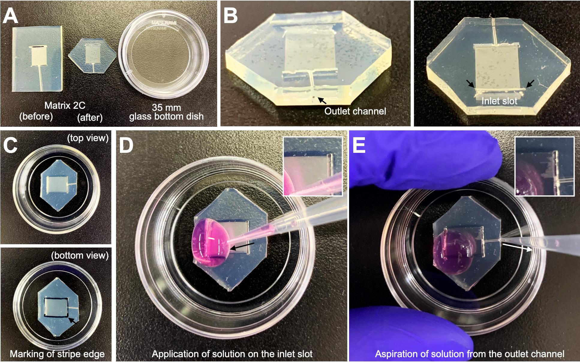
Figure 1. Preparation of stripes on a 35 mm glass-bottom dish. (A) Representative images showing Matrix 2C before and after corner cutting alongside a 35 mm glass-bottom dish. The corners of Matrix 2C are trimmed with a blade to fit within the glass-bottom dish. (B) Close-up views of the outlet channel and inlet slot (arrows) of the corner-cut Matrix 2C. (C) Top and bottom views of the dish with the corner-cut Matrix 2C attached. The stripe edge is marked on the glass surface as indicated by the arrow in the bottom view. (D, E) Critical steps for stripe preparation. A solution is applied to the inlet slot (D) and aspirated through the outlet channel using a P200 pipette. During the initial aspiration (step C4), the penetration of the solution into the stripe lanes is visible (D and E, boxed area).
2. Attach Matrix 2C to a 35 mm glass-bottom dish. Mark the edges of the stripe area on the glass surface (Figure 1C).
3. Put 200 μL of ice-cold Sdc2/BSA-alexa647 solution around the inlet slot (Figure 1D).
4. Aspirate air and solution from the outlet channel using a P200 pipette to fill the solution inside the Matrix 2C at RT (Figure 1E).
Critical: Air bubbles inside the stripe lanes should be removed by aspiration.
5. Repeat steps C3 and C4 5–6 times.
6. Incubate the dish with Matrix 2C for 30 min at 37 °C.
7. Collect all the solution from the Matrix 2C with a P200 pipette.
Note: Sdc2/BSA-alexa647 solution can be repeatedly used for two weeks.
8. Put 200 μL of ice-cold L15 medium around the inlet slot (Figure 1D).
9. Aspirate air and solution using a P200 pipette to wash the stripe lanes inside the Matrix 2C (Figure 1E).
10. Repeat steps C8 and C9 10 times.
11. Detach the Matrix 2C from the dish.
12. Dry the dish for 5 min.
13. Embed the cell aggregates with ice-cold 60% Matrigel/Ncan/L15 medium on the Sdc2-stripes.
Proceed with further steps as described previously (step D16 from [8]).
D. Nucleofection of migrating V-SVZ-derived neurons
Note: Use the AmaxaTM P3 Primary Cell 4D-NucleofectorTM X kit for the following procedures.
1. Obtain V-SVZ-derived cells from P0-1 pups (four pups per experimental group) in ice-cold L15 medium as previously described (steps B1–C9 from [8]).
2. Prepare Nucleofector® solution (see manufacturer’s instructions).
3. Add 100 μL of the Nucleofector solution at RT to the cell pellet and suspend the cells gently.
4. Mix the cell suspension with plasmid(s) (maximum total plasmid amount is 2.0 μg per tube).
5. Transfer the cell suspension into the supplied single nucleocuvette. Place the cuvette into the Amaxa 4D-Nucleofector X Unit and run the program CL-133.
6. Incubate the cell suspension for 10 min at RT and add 400 μL of prewarmed RPMI-1640 medium.
7. Transfer the cell suspension to a fresh tube using the supplied plastic pipette.
8. Spin down the tube for 1 min and remove the supernatant.
Proceed with further steps as described above (step D9 from [8]).
E. Fixation and immunocytochemical staining of cultured neurons
1. Prewarm (37 °C) 4% PFA in 0.1 M PB (pH 7.4) in a bead bath.
2. Remove the culture medium (NB final medium or DMEM culture medium) using an aspirator and immediately (within 3 s) incubate the cells with 300 μL of prewarmed 4% PFA in 0.1 M PB for 15 min at 37 °C.
Critical: Make sure to strictly maintain a temperature of 37 °C during this step for the maintenance of cytoskeletal organization in the growth cone.
3. Wash the cells with 500 μL of PBS at RT for 5 min.
4. Repeat step E3 three times.
5. Incubate the cells with 200 μL of blocking solution for 30 min at RT.
6. Incubate the cells with 200 μL of primary antibody diluted in blocking solution overnight at 4 °C. For F-actin staining, use Alexa Fluor-conjugated phalloidin.
7. Wash the cells with 500 μL of PBS/0.2% Triton X-100 for 5 min.
8. Repeat step E7 three times.
9. Incubate the cells with 200 μL of AlexaFluor-conjugated secondary antibody diluted in blocking solution for 2 h at RT.
10. Wash the cells with 500 μL of PBS for 5 min.
11. Repeat step E10 three times.
12. Mount a coverslip on the slide glass with mounting medium. Carefully tilt the coverslip to distribute the mounting medium evenly between the specimen and the coverslip without making bubbles.
F. Super-resolution imaging of growth cones in fixed neurons
1. Start up the super-resolution microscope system and the operation software.
2. Choose cells of interest. We usually choose target cells that show active migration and are located far from the V-SVZ cell aggregates (>200 μm).
3. Choose an objective lens. 40× water-immersion and 63× oil-immersion objective lenses are preferable for the acquisition of whole cell morphology and growth cone, respectively.
Critical: Imaging target cells far from the cell aggregates can avoid autofluorescence from the aggregates.
4. Set the laser powers and detector gains, which depend on the status of microscope systems and laser output. The excitation wavelengths of the lasers used in this study are as follows: 405 nm for Hoechst 33342, 488 nm for Alexa488, 561 nm for Alexa594, and 633 nm for Alexa647. In our microscope system, the fiber outputs of the 405 nm, Argon (500 nm), 561 nm, and 633 nm lasers are 15.08, 12.33, 3.31, and 1.04 mW, respectively, and illumination laser powers are set to 1.0%–3.0% (405, 488, 561, and 633 nm).
Critical: Since the brightness and resistance to photobleaching can also vary among fluorescent proteins/probes, the appropriate range of laser power for each experimental condition should be manually optimized by the researcher. The laser power should be minimized as much as possible while maintaining a high signal-to-noise ratio to avoid photobleaching.
5. Set the X/Y/Z resolutions. For image acquisition of cytoskeletal networks and cellular protrusions, 0.040–0.050 μm/pixel in X/Y resolution is preferable. In our study, the optical zoom is set to 1.8× and 3.0× for 40× water-immersion and 63× oil-immersion objective lenses, respectively. For the acquisition of the three-dimensional organization of cytoskeletal molecules, 0.18–0.30 μm/z-plane in Z resolution is preferable. Optimal setting mode is also useful for automatically setting appropriate X/Y/Z resolutions in any setting of optical zoom and objective lens.
6. Set the pixel dwell time. We set 3.52 μs/pixel for super-resolution imaging of fixed neurons [7], whose values depend on the status of microscope systems and laser output. For better image acquisition, use an “average” scanning mode.
7. Start image acquisition.
8. Save the image file in a format specified by the microscope supplier (.czi for Carl Zeiss ZEN software).
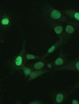
10. Process the saved file to make super-resolution images. In the case of the Carl Zeiss LSM880 system, the Airyscan processing function is used (Figure 2).
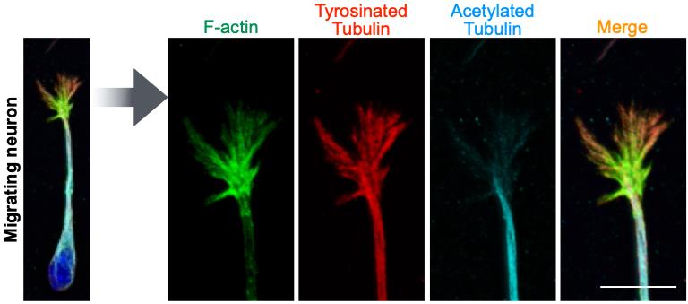
Figure 2. Subcellular distribution of cytoskeletal molecules in the growth cone of fixed migrating neurons. Representative super-resolution images of ventricular–subventricular zone (V-SVZ)-derived cultured neurons stained for F-actin (green), tyrosinated tubulin (a marker for dynamic microtubules, red), and acetylated tubulin (a marker for stable microtubules, light blue). The nucleus is stained with Hoechst 33342 (blue). The growth cone is magnified in the right panels. In the growth cone, while F-actin and tyrosinated tubulin+ fibrous signals are observed in the central and peripheral domains, acetylated tubulin is observed only in the central domain. Scale bar, 5 μm.
G. Super-resolution time-lapse imaging of growth cones in living neurons
1. Pre-incubate the stage-top incubation chamber at 37 °C with 5% CO2 (without cells) for 1 h to stabilize the system.
2. Set a 35 mm glass-bottom dish containing cultured neurons in the stage-top incubation chamber for 1 h (Figure 3A).
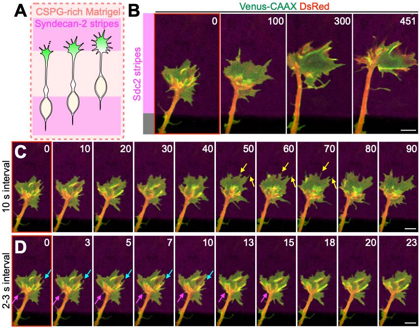
Figure 3. Dynamics of leading process growth cone on the Sdc2-coated stripe in the presence of CSPG. (A) Experimental scheme. CSPG-rich Matrigel corresponds to 60% Matrigel/Ncan/L15 medium. (B–D) Representative super-resolution time-lapse images of ventricular–subventricular zone (V-SVZ)-derived cultured migrating neurons expressing Venus-CAAX (green) and DsRed (red), which label membranes and cytosol, respectively. While “minute-interval” imaging reveals the overall dynamics of the leading process growth cone (B), “second-interval” imaging visualizes the dynamics of fine cellular structures such as lamellipodia and filopodia. (C, D) Yellow, light-blue, and magenta arrows indicate formed, buried, and retracted filopodium, respectively. The structure and dynamics of lamellipodial and filopodial structures should be additionally analyzed by using actin probes such as GFP-actin or EGFP-UtrCH. Numbers indicate seconds from the first imaging frame (B–D). Scale bars, 5 μm (B–D). CSPG, chondroitin sulfate proteoglycan.
3. Choose an objective lens. 40× water-immersion and 63× oil-immersion objective lenses are preferable for the acquisition of whole cell morphology and growth cone, respectively. In the case of the 40× objective lens, use lens oil with a refractive index equivalent to water to avoid water evaporation on the objective lens in long-term time-lapse imaging.
4. Set the laser powers and detector gains, which depend on the status of microscope systems and laser output. The excitation wavelengths of lasers used in this study are as follows: 488 nm for GFP/Venus, 561 nm for DsRed/tdTomato, and 633 nm for Alexa647. In our microscope system, the fiber outputs of the 405 nm, Argon (500 nm), 561 nm, and 633 nm lasers are 15.08, 12.33, 3.31, and 1.04 mW, respectively, and illumination laser powers are set to 1.0%–3.0% (405, 488, 561, and 633 nm).
Critical: Since the brightness and resistance to photobleaching can also vary among fluorescent proteins/probes, the appropriate range of the laser power for each experimental condition should be manually optimized by the researcher. The laser power should be minimized as much as possible while maintaining a high signal-to-noise ratio to avoid photobleaching.
5. Set the X/Y/Z resolutions. For image acquisition of cytoskeletal networks and cellular protrusions, 0.040–0.050 μm/pixel in X/Y resolution is preferable. In our study, the optical zoom is set as 1.8× and 3.0× for 40× water-immersion and 63× oil-immersion objective lenses, respectively. For the acquisition of three-dimensional organization of cytoskeletal molecules and cell morphology, 0.18–0.30 μm/z-plane (0.189 μm in our study) and 0.5–1.0 μm/z-plane (1.0 μm in our study), respectively, in Z resolution is preferable. Optimal setting mode is also useful to automatically set appropriate X/Y/Z resolutions in any setting of optical zoom and objective lens.
6. Set the pixel dwell. We set 0.74 and 0.99 μs/pixel for super-resolution imaging of living neurons and their growth cones, respectively [7], whose values depend on the status of microscope systems and laser output. For better image acquisition, use an “average” scanning mode.
7. Set the time interval (Figure 3B–D). In our study [7], for the acquisition of cell behaviors, we set the interval to 30 s per frame. For the acquisition of cytoskeletal dynamics (F-actin and microtubule polymerization) in the growth cone, set the interval to 3.0–6.0 s per frame.
8. Use a focus drift compensation system if the microscope possesses it. In our study, we use the Definite Focus 2 function (Carl Zeiss) in every imaging frame to avoid focus drift during time-lapse imaging.
9. Find the targeted cell.
Critical: Make sure to target a cell that directly adheres, or is located very close, to the cover glass. Targeting a cell that is far from the cover glass will drastically reduce the spatial resolution in super-resolution imaging.
10. Start image acquisition. Frequently check whether phototoxicity or photobleaching occurs.
Critical: In our imaging, photobleaching is determined by the rapid decrease of fluorescent intensity, and phototoxicity is determined by the rapid decrease of cellular motility and disruption of morphology. In case of phototoxicity or photobleaching, reduce the values of laser power, pixel dwell, and/or average scanning number, and/or extend the imaging interval.
11. Save the image file in a format specified by the microscope supplier (.czi for Carl Zeiss ZEN software).
12. Process the saved file to make super-resolution images. In the case of the Carl Zeiss LSM880 system, the Airyscan processing function is used.
H. Optical manipulation of cytoskeletal molecules in super-resolution time-lapse imaging
1. Pre-incubate the stage-top incubation chamber at 37 °C with 5% CO2 (without cells) for 1 h to stabilize the system.
2. Set a 35 mm glass-bottom dish containing cultured neurons and photoactivatable inhibitors in the stage-top incubation chamber for 1 h. In our study, Opto-Lat, PnOJ, and PST-1 are added to the medium at the final concentration of 5.0, 0.4, and 2.0 μM, respectively (Figure 4).
Critical: Make sure to keep the dish under dark conditions throughout the experiment.
Critical: Ensure there is no effect of photoswitchable inhibitors on growth cone dynamics under dark conditions.
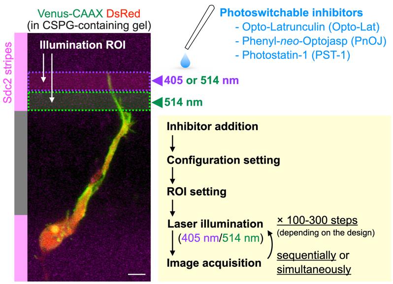
Figure 4. Experimental scheme for optical manipulation of cytoskeletal molecules using photoswitchable inhibitors. Following inhibitor addition to the media, the configuration and illumination ROI is quickly set. Laser illumination for inhibitor activation/inactivation and image acquisition are performed sequentially or simultaneously, depending on microscope specifications.
3. Set the imaging configuration in the microscope system according to steps G3–8 (Figure 4).
4. Set the ROI for targeted illumination in the microscope system (Figure 4). In our study, the squared ROI for 405 nm laser illumination is set on the targeted region (4 μm width) to activate photoactivatable inhibitors. Moreover, we set the squared ROI for 514 nm laser illumination in the neighboring region to suppress the activity of potentially diffusing activated inhibitors.
5. Set the illumination power of 405 and 514 nm lasers. Laser power is determined by the inhibitory activity of activated inhibitors on actin and microtubule dynamics. In our microscope system, the fiber outputs of the 405 nm and Argon (500 nm) lasers are 15.08 and 12.33 mW, respectively, and illumination laser powers are set to 2.0% (405 and 514 nm).
6. Set the illumination duration. Detailed settings configuration depends on the microscope system. In the case of Carl Zeiss LSM880, we use bleaching iteration mode and set it to 20, which leads to 6–8 s illumination.
7. Set the baseline imaging session. In our study, 5–10 frames, which depends on the experiment, are acquired before starting laser illumination.
8. Start image acquisition. Laser illumination for inhibitor activation and image acquisition can be simultaneously or sequentially performed (Figure 4).
9. Save the image file in a format specified by the microscope supplier (.czi for Carl Zeiss ZEN software).
10. Process the saved file to make super-resolution images. In the case of the Carl Zeiss LSM880 system, the Airyscan processing function is used.
I. Machine learning–based segmentation of axonal and leading process growth cone area
1. Prepare z-stack projection images of growth cones in axons (training datasets).
2. Open z-stack projection images via FIJI and select the Trainable Weka Segmentation plugin from Plugins > Segmentation.
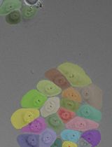
3. Draw freehand lines on the axonal growth cone, shaft, and background in an arbitrary frame and classify them into classes 1, 2, and 3, respectively (Figure 5A).
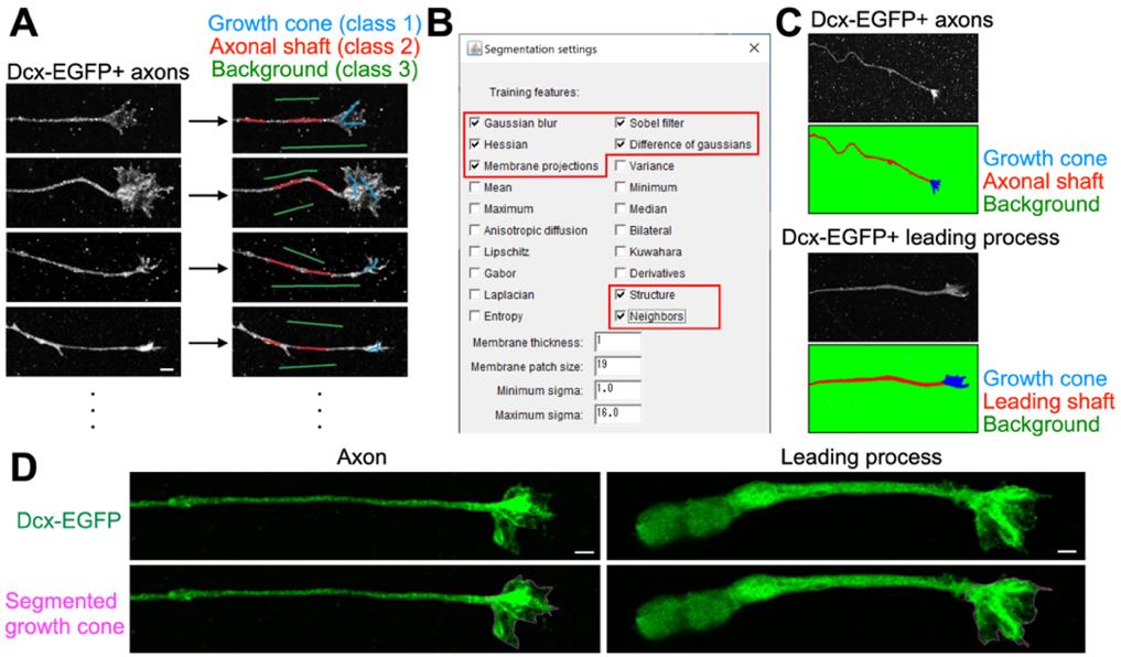
Figure 5. Machine learning–based segmentation of growth cone area in axons and leading processes of cultured neurons. (A) Training of segmentation of growth cone area using the Trainable Weka Segmentation plugin (FIJI). The axonal image is classified into growth cone (light blue), axonal shaft (red), and background (green). (B) Selection of training features in the Trainable Weka Segmentation plugin. Users should choose appropriate features by trial and error. (C, D) Successful segmentation of growth cone area in axons and leading process. Axonal and leading process growth cone areas are shown in blue (C) and dotted lines (D). Scale bars, 2 μm.
4. Repeat step I3 for nine images per cell (for time-lapse images) or nine other cells (for fixed neuron images).
5. Select the training features (Gaussian blur, Hessian, Membrane projections, Sobel filter, Difference of Gaussians, Structure, and Neighbors) in the Settings of the Trainable Weka Segmentation window (Figure 5B). Other features (Mean, Variance, Median, Minimum, Maximum Anisotropic diffusion, Bilateral, Lipschitz, Kuwahara, Gabor, Derivatives, Laplacian, and Entropy) can additionally be used depending on the experimental conditions.
6. Select Train classifier in the Trainable Weka Segmentation window.
7. Repeat steps I3–6 for 4–6 cells (for time-lapse images).
8. Select Save classifier to save the algorithm.
9. Prepare z-stack projection images of growth cones in the leading process of migrating neurons (test datasets).
Critical: Fluorescent proteins, image acquisition setting, and x/y resolution in images must be completely identical to training datasets.
10. Open z-stack projection images via FIJI and select the Trainable Weka Segmentation plugin from Plugins > Segmentation.
11. Select Load classifier to open the algorithm.
12. Select Create result to perform segmentation of the leading process images into growth cone, shaft, and background (Figure 5C, D).
13. Save the image file.
14. In case of the quantification of growth cone area and/or density, use the Analyze Particle tool from the Analyze tab. Analyzed components can be selected from the Set Measurements tool from the Analyze tab.
Caution: These quantification analyses are highly variable depending on the purpose, experimental setting, and image acquisition conditions, and should be manually established by each researcher. Detailed manuals or instructions for the FIJI plugins are available on the website.
J. Analyses of lamellipodial and filopodial dynamics in time-lapse super-resolution images of growth cones
1. Open time-lapse images of growth cones in the microscope supplier’s software (e.g., ZEN for Carl Zeiss). For lamellipodial and filopodial dynamics analyses in our study, GFP-actin images are used. For analyses of microtubule polymerization, EB3-EGFP images are used.
2. For lamellipodial and filopodial dynamics analyses, define the degree in the growth cone (axonal shaft is set to -90°).
3. Filopodia dynamics is classified into three types: formed filopodia, retracted filopodia, and buried filopodia. Filopodia is defined as an GFP-actin+ spike-like structure formed from the growth cone.
Note: Typical examples of formed, retracted, and buried filopodia in membrane time-lapse imaging are shown in Figure 3C and 3D. For a detailed analysis of these structures and dynamics, use actin probes.
4. Record the degree of all filopodial events in the growth cone every 20th frame for >300 s in the microscope supplier’s software (e.g., ZEN for Carl Zeiss).
Note: Researchers can set additional parameters, such as filopodial extension speed (μm/min) and persistence (min/filopodium).
5. Record the degree of the formed lamellipodial events in the growth cone from at least 100 sequential frames. Lamellipodium is defined as GFP-actin+ membrane extension observed between two formed filopodia.
Note: Researchers can set additional parameters, such as lamellipodial extension speed (μm/min) and persistence (min/lamellipodium).
6. For analysis of microtubule polymerization within the filopodia, record the density of EB3-EGFP+ dots in the resting and extending growth cone.
K. Analyses of the effects of photoswitchable inhibitors on F-actin and microtubule dynamics in time-lapse super-resolution images of growth cones
1. Open time-lapse images of growth cones in the microscope supplier’s software (e.g., ZEN for Carl Zeiss).
2. For analysis of the effect of Opto-Lat activation on F-actin polymerization in the Sdc2 stripe assay in 514 and 405 nm groups, measure the EGFP-UtrCH+ F-actin intensity in filopodia (within the targeted ROI) and leading shaft (as an internal control) using the function of the microscope supplier’s software (e.g., ZEN for Carl Zeiss) for 2–4 min from their invasion into the Sdc2 stripe. For analysis of the effect of PnOJ activation, do the same for 4–6 min from their invasion into the Sdc2 stripe.
Critical: Since the EGFP-UtrCH+ F-actin intensity is highly variable among cells due to varied transfection efficiency, internal control measurement (leading shaft in our case) is required. Set the region of internal control outside of the target region of Opto-Lat activation.
3. For analysis of the effect of PST-1 activation on microtubule polymerization in the Sdc2 stripe assay in 514 and 405 nm groups, measure the EB3-EGFP+ dot density in filopodia (within the targeted ROI) and leading shaft (as an internal control) using the function of the microscope supplier’s software (e.g., ZEN for Carl Zeiss) for 2–4 min from their invasion into Sdc2 stripe.
Critical: Since the EB3-EGFP+ dot number is highly variable among cells due to varying transfection efficiency, internal control measurement (leading shaft in our case) is required. Set the region of internal control outside of the target region of PST-1 activation.
4. Obtained numerical data is normalized, which enables one to compare different experimental groups. In our case, we set the EGFP-UtrCH+ intensity or EB3-EGFP+ dot density in the leading filopodium in the 514 nm group to 1 (Supplementary Figure 4g [7]).
Validation of protocol
This protocol has been used and validated in the following research article:
• Nakajima et al. [7]. Identification of the growth cone as a probe and driver of neuronal migration in the injured brain. Nature Communications (Figure 1, panels a–n; Figure 2, panels b, c, l–m; Figure 3, panels b–f)
Acknowledgments
This protocol was used in [7]. We thank K. Kaibuchi (Fujita Health University, Japan), H. Nakagawa (Nagoya City University, Japan), W. Bement (University of Wisconsin-Madison), and D.J. Solecki (St. Jude Children’s Research Hospital) for materials; the Research Equipment Sharing Center JPMXS0441500024 and the Center for Experimental Animal Science at Nagoya City University for providing technical and animal support; and Sawamoto laboratory members for discussions. This work was supported by research grants from Japan Agency for Medical Research and Development (AMED) [24gm1210007, 21bm0704033h0003 (to K.S.) and 21jm0210060 (to K.S., and M.S.)], Japan Society for the Promotion of Science (JSPS) KAKENHI [26250019, 17H01392, 19H04785, 18KK0213, 20H05700, and JP22H04926 to K.S.), 21K06395 and 24K09660 (to M.S.), and 23K19406 (to C.N.)] and Core-to-Core Program (JPJSCCA20230007, to K.S.), Bilateral Open Partnership Joint Research Projects (to K.S.), Grant-in-Aid for Research at Nagoya City University (to K.S. and M.S.), Grant-in-Aid for Outstanding Research Group Support Program in Nagoya City University (2401101, to K.S.), Grant-in-Aid for Promotion on Co-Creative Urban Development in Nagoya City University (2412145, to K.S.), the Deutsche Forschungsgemeinschaft [Cluster of Excellence EXC2051 Balance of the Microverse—Microverse—Project-ID 390713860, equipment grant INST 275/442-1 FUGG (to H.-D.A.)], Deutscher Akademischer Austauschdienst (to V.N. and H.-D.A.), Studienstiftung des deutschen Volkes (to N.A.V.), the Mitsubishi Foundation (to K.S.), the Canon Foundation (to K.S.), the Nitto Foundation (to M.S.), the Hori Science & Arts Foundation (to M.S.), Terumo Life Science Foundation (M.S.), and the Takeda Science Foundation (to K.S. and M.S.).
Competing interests
The authors declare no competing interests.
Ethical considerations
All protocols in this study were performed in accordance with the guidelines and regulations of Nagoya City University (animal protocol number 21-028; gene recombination protocol numbers 23-119 and 22-133).
References
- Stoeckli, E. T. (2018). Understanding axon guidance: are we nearly there yet? Development 145(10): e151415. https://doi.org/10.1242/dev.151415
- Cajal, S. R. (1890). A quelle époque apparaissent les expansions des cellules nerveuses de la moelle épinière du poulet. Anat Anz. 5: 609–613.
- Lowery, L. A. and Vactor, D. V. (2009). The trip of the tip: understanding the growth cone machinery. Nat Rev Mol Cell Biol. 10(5): 332–343. https://doi.org/10.1038/nrm2679
- Kaneko, N., Sawada, M. and Sawamoto, K. (2017). Mechanisms of neuronal migration in the adult brain. J Neurochem. 141(6): 835–847. https://doi.org/10.1111/jnc.14002
- He, M., Zhang, Z. h., Guan, C. b., Xia, D. and Yuan, X. b. (2010). Leading Tip Drives Soma Translocation via Forward F-Actin Flow during Neuronal Migration. J Neurosci. 30(32): 10885–10898. https://doi.org/10.1523/jneurosci.0240-10.2010
- Jiang, J., Zhang, Z. H., Yuan, X. B. and Poo, M. M. (2015). Spatiotemporal dynamics of traction forces show three contraction centers in migratory neurons. J Cell Biol. 209(5): 759–774. https://doi.org/10.1083/jcb.201410068
- Nakajima, C., Sawada, M., Umeda, E., Takagi, Y., Nakashima, N., Kuboyama, K., Kaneko, N., Yamamoto, S., Nakamura, H., Shimada, N., et al. (2024). Identification of the growth cone as a probe and driver of neuronal migration in the injured brain. Nat Commun. 15(1): e1038/s41467–024–45825–8. https://doi.org/10.1038/s41467-024-45825-8
- Sawada, M., Matsumoto, M., Narita, K., Kumamoto, N., Ugawa, S., Takeda, S. and Sawamoto, K. (2020). In vitro Time-lapse Imaging of Primary Cilium in Migrating Neuroblasts. Bio Protoc. 10(22): e3823. https://doi.org/10.21769/bioprotoc.3823
- Vepřek, N. A., Cooper, M. H., Laprell, L., Yang, E. N., Folkerts, S., Bao, R., Boczkowska, M., Palmer, N. J., Dominguez, R., Oertner, T. G., et al. (2024). Optical Control of G-Actin with a Photoswitchable Latrunculin. J Am Chem Soc. 146(13): 8895–8903. https://doi.org/10.1021/jacs.3c10776
- Küllmer, F., Vepřek, N. A., Borowiak, M., Nasufović, V., Barutzki, S., Thorn‐Seshold, O., Arndt, H. and Trauner, D. (2022). Next Generation Opto‐Jasplakinolides Enable Local Remodeling of Actin Networks. Angew Chem Int Ed. 61(48): e202210220. https://doi.org/10.1002/anie.202210220
- Borowiak, M., Nahaboo, W., Reynders, M., Nekolla, K., Jalinot, P., Hasserodt, J., Rehberg, M., Delattre, M., Zahler, S., Vollmar, A., et al. (2015). Photoswitchable Inhibitors of Microtubule Dynamics Optically Control Mitosis and Cell Death. Cell. 162(2): 403–411. https://doi.org/10.1016/j.cell.2015.06.049
- Watanabe, T., Kakeno, M., Matsui, T., Sugiyama, I., Arimura, N., Matsuzawa, K., Shirahige, A., Ishidate, F., Nishioka, T., Taya, S., et al. (2015). TTBK2 with EB1/3 regulates microtubule dynamics in migrating cells through KIF2A phosphorylation. J Cell Biol. 210(5): 737–751. https://doi.org/10.1083/jcb.201412075
- Burkel, B. M., von Dassow, G. and Bement, W. M. (2007). Versatile fluorescent probes for actin filaments based on the actin‐binding domain of utrophin. Cell Motil. 64(11): 822–832. https://doi.org/10.1002/cm.20226
- Knöll, B., Weinl, C., Nordheim, A. and Bonhoeffer, F. (2007). Stripe assay to examine axonal guidance and cell migration. Nat Protoc. 2(5): 1216–1224. https://doi.org/10.1038/nprot.2007.157
- Schindelin, J., Arganda-Carreras, I., Frise, E., Kaynig, V., Longair, M., Pietzsch, T., Preibisch, S., Rueden, C., Saalfeld, S., Schmid, B., et al. (2012). Fiji: an open-source platform for biological-image analysis. Nat Methods. 9(7): 676–682. https://doi.org/10.1038/nmeth.2019
- Kanda, Y. (2012). Investigation of the freely available easy-to-use software ‘EZR’ for medical statistics. Bone Marrow Transplant. 48(3): 452–458. https://doi.org/10.1038/bmt.2012.244
- Beaudoin, G. M. J., Lee, S. H., Singh, D., Yuan, Y., Ng, Y. G., Reichardt, L. F. and Arikkath, J. (2012). Culturing pyramidal neurons from the early postnatal mouse hippocampus and cortex. Nat Protoc. 7(9): 1741–1754. https://doi.org/10.1038/nprot.2012.099
Article Information
Publication history
Received: Nov 10, 2024
Accepted: Feb 14, 2025
Available online: Mar 9, 2025
Published: Mar 20, 2025
Copyright
© 2025 The Author(s); This is an open access article under the CC BY-NC license (https://creativecommons.org/licenses/by-nc/4.0/).
How to cite
Sawada, M., Nakajima, C., Umeda, E., Takagi, Y., Nakashima, N., Vepřek, N. A., Küllmer, F., Nasufović, V., Arndt, H., Trauner, D., Igarashi, M. and Sawamoto, K. (2025). Time-Lapse Super-Resolution Imaging and Optical Manipulation of Growth Cones in Elongating Axons and Migrating Neurons. Bio-protocol 15(6): e5251. DOI: 10.21769/BioProtoc.5251.
Category
Neuroscience > Cellular mechanisms > Cell isolation and culture
Cell Biology > Cell imaging > Live-cell imaging
Do you have any questions about this protocol?
Post your question to gather feedback from the community. We will also invite the authors of this article to respond.