- Protocols

- Articles and Issues
- For Authors
- About
- Become a Reviewer

Monitoring Changes in Intracellular Chloride Levels Using the FRET-Based SuperClomeleon Sensor in Organotypic Hippocampal Slices
Published: Vol 15, Iss 5, Mar 5, 2025 DOI: 10.21769/BioProtoc.5229 Views: 2858
Reviewed by: Marco Di GioiaThirupugal GovindarajanAndrea GramaticaDavide Pallucci
Original research article
The authors used this protocol in:

Jan 2023
Advertisement


Protocol Collections
Comprehensive collections of detailed, peer-reviewed protocols focusing on specific topics


Abstract
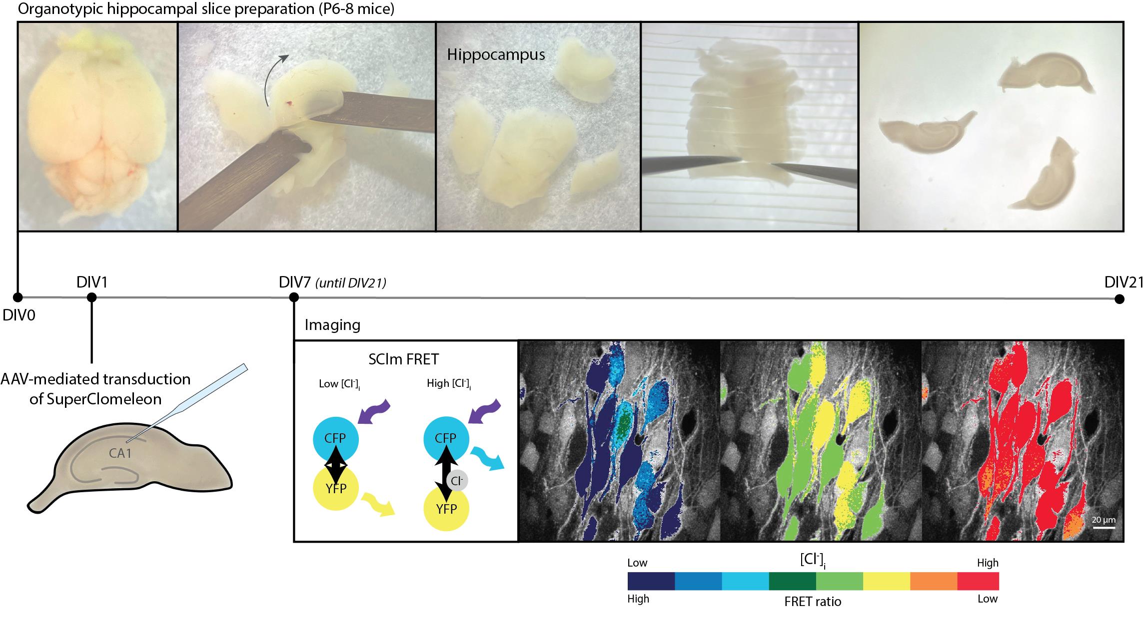
The reduction in intracellular neuronal chloride concentration is a crucial event during neurodevelopment that shifts GABAergic signaling from depolarizing to hyperpolarizing. Alterations in chloride homeostasis are implicated in numerous neurodevelopmental disorders, including autism spectrum disorder (ASD). Recent advancements in biosensor technology allow the simultaneous determination of intracellular chloride concentration of multiple neurons. Here, we describe an optimized protocol for the use of the ratiometric chloride sensor SuperClomeleon (SClm) in organotypic hippocampal slices. We record chloride levels as fluorescence responses of the SClm sensor using two-photon microscopy. We discuss how the SClm sensor can be effectively delivered to specific cell types using virus-mediated transduction and describe the calibration procedure to determine the chloride concentration from SClm sensor responses.
Key features
• Calibration and use of the ratiometric chloride sensor SuperClomeleon to measure intracellular chloride levels in mouse organotypic hippocampal slices.
• SuperClomeleon sensor expression in pyramidal cells or GABAergic interneurons using adeno-associated viruses.
Keywords: SuperClomeleonGraphical overview
Background
Chloride ions are involved in the regulation of many basic cellular properties, including cell volume, intracellular pH, and membrane potential. Defects in chloride homeostasis occur in many diseases, including neurodevelopmental disorders. In neurons, chloride mediates synaptic signaling. While GABA is the main inhibitory neurotransmitter in the adult brain, during early development, GABAergic signaling is excitatory, which aids proper wiring of the developing brain [1,2]. The transition of GABAergic action from depolarizing to hyperpolarizing later in development is called the GABA shift. A disturbance of the GABA shift is implicated in various neurodevelopmental disorders [2–5]. The GABA shift is the result of a delayed expression of the chloride exporter KCC2 in developing neurons, while immature neurons already express the chloride importer NKCC1 [1]. As a consequence, intracellular chloride concentrations are high in immature neurons, while healthy adult neurons maintain low chloride levels. To characterize the GABA shift during brain development, or to assess changes in chloride homeostasis in the context of diseases, a reliable method to determine intracellular chloride concentrations is indispensable.
A reliable method to determine the intracellular chloride concentration in individual neurons is performing perforated patch clamp recordings using selective cation-permeable ionophores [6,7]. This technique is technically difficult to perform and time-intensive, resulting in a relatively low yield. As there is ample variability between individual cells, a high number of experiments is required in order to draw conclusions on the population level. Recent technological advancements in biosensors, more specifically in chloride sensors, are now providing a promising high-throughput alternative, in which intracellular chloride levels can be monitored without interference of the intracellular milieu. There are several chloride sensors currently under development, each with specific advantages and disadvantages [8].
Early chemical chloride sensors lacked the ability to target specific groups of cells, while single color-based genetically encoded chloride sensors are sensitive to variations in the local concentration of the sensor [9]. Fluorescence resonance energy transfer (FRET)-based sensors circumvent these issues as their expression can be targeted to specific cell types using the Cre-Lox system and their ratiometric properties allow the determination of chloride concentration independently of sensor concentration [8,9]. The FRET sensor SuperClomeleon (SClm) is an improved version of the first genetically encoded ratiometric chloride sensor Clomeleon. It provides enhanced chloride sensitivity and is well-suited for the simultaneous imaging of chloride levels in many neurons [8,10,11]. SClm contains two fluorescent proteins, Cerulean (CFP mutant) and Topaz (YFP mutant), which are joined together by a flexible linker region [11]. FRET occurs between the CFP donor and the YFP acceptor when chloride is not bound, whereas no FRET occurs when chloride is bound to the sensor. In this way, the FRET ratio (YFP/CFP fluorescence intensity) indicates the intracellular chloride concentration. The SClm sensor has been successfully employed to study the contribution of NKCC1 and the WNK pathway to chloride homeostasis in neuronal cultures [12], to determine steady-state intracellular chloride concentration in cortical neurons in vivo [13], and to demonstrate chloride microdomains in hippocampal pyramidal neurons [14], illustrating its broad applicability. We recently used SClm to monitor developmental changes in intraneuronal chloride concentration in organotypic hippocampal slices [15]. In the current protocol, we provide a detailed description of how to optimize and calibrate SClm for determining intracellular chloride concentration in developing organotypic hippocampal slices. SClm expression in pyramidal cells and interneurons was achieved via virus-mediated transduction. We provide a step-by-step description of the preparation of slice cultures and virus injection and describe the two-photon microscopy and image analysis. Lastly, we discuss how to properly calibrate the sensor to determine intracellular chloride concentrations from measured FRET ratios.
Materials and reagents
Biological materials
1. C57BL/6 wild-type mice (The Jackson Laboratory, strain #000664)
2. C57BL/6 VGAT-Cre mice B6J.129S6(FVB)-Slc32a1tm2(cre)Lowl/MwarJ (The Jackson Laboratory, strain #028862)
Note: VGAT is the vesicular GABA transporter (encoded by the Slc32a1 gene). VGAT-Cre mice allow targeted expression of the SuperClomeleon sensor in (VGAT-expressing) interneurons.
3. Floxed SuperClomeleon construct under the control of synapsin promotor (a gift from prof. dr. Thomas Kuner, Heidelberg University, Germany)
4. Non-floxed SuperClomeleon construct under the control of the synapsin promotor (a gift from Kevin Staley, Massachusetts General Hospital, Boston, MA)
Note: Different SClm constructs are now commercially available from the Addgene website: https://www.addgene.org/browse/article/28244285/
Reagents
1. Calcium chloride (CaCl2) (Merck, catalog number 102382)
2. D-(+)-glucose (Sigma-Aldrich, catalog number: G7528)
3. Ethylene glycol-bis(β-aminoethyl ether)-N,N,N',N'-tetraacetic acid (EGTA) (Sigma-Aldrich, catalog number: E4378)
4. Hanks’ balanced salt solution (HBSS) (Gibco, catalog number: 24020-091)
5. HEPES (Sigma-Aldrich, catalog number: H4034)
6. Horse serum (Gibco, catalog number: 26050-088)
7. K-gluconate (Sigma-Aldrich, catalog number: P1847)
8. Kynurenic acid (Sigma-Aldrich, catalog number: K3375)
9. Magnesium chloride (MgCl2) (Sigma-Aldrich, catalog number: M2670)
10. Magnesium sulfate (MgSO4) (Sigma-Aldrich, catalog number: 63138)
11. Mg(gluconate)2 (Sigma-Aldrich, catalog number: G9130)
12. MgATP (Carbosynth, catalog number: NA44288)
13. Minimal essential medium 1× (MEM) (Gibco, catalog number: 11575-032)
14. Na2-phosphocreatine (Sigma-Aldrich, catalog number: P7936)
15. NaF (Sigma-Aldrich, catalog number: 201154)
16. Na-gluconate (Sigma-Aldrich, catalog number: S2054)
17. NaGTP (Sigma-Aldrich, catalog number: G8877)
18. Nigericin (Sigma-Aldrich, catalog number: N7143)
19. Phosphate buffered saline (PBS), pH 7.2, 1× (Gibco, catalog number: 20012027)
20. Potassium chloride (KCl) (Sigma-Aldrich, catalog number: P5405)
21. Potassium fluoride (KF) (Thermo Scientific, catalog number: 42216)
22. Potassium phosphate monobasic (KH2PO4) (Sigma-Aldrich, catalog number: P5655)
23. Sodium chloride (NaCl) (Sigma-Aldrich, catalog number: S7653)
24. Sodium dihydrogen phosphate (NaH2PO4) (Merck, catalog number: A977446)
25 Sodium hydrogen carbonate (NaHCO3) (Merck, catalog number: 106329)
26. Tributyltin acetate (Merck, catalog number: 821650)
27. Trolox (Acros Organics, catalog number: 218940250)
Solutions
1. Gey’s balanced salt solution (GBSS) (see Recipes)
2. Culture medium (see Recipes)
3. Artificial cerebrospinal fluid (ACSF) (see Recipes)
4. High chloride solution (see Recipes)
5. Low chloride solution (see Recipes)
6. KF quenching solution (see Recipes)
Recipes
1. Gey’s balanced salt solution (GBSS) (50 mL)
Note: Osmolarity should be 325 ± 5 mOsm. Add sucrose to increase osmolarity if needed. pH should be 7.3–7.4.
| Reagent | Final concentration |
| NaCl | 137 mM |
| KCl | 1.5 mM |
| CaCl2 | 1.5 mM |
| MgCl2 | 1 mM |
| MgSO4 | 0.3 mM |
| KH2PO4 | 0.2 mM |
| Na2HPO4 | 0.85 mM |
| D-(+)-glucose | 25 mM |
| HEPES | 12.5 mM |
| Kynurenic acid | 1 mM |
2. Culture medium (50 mL)
Note: Osmolarity should be 325 ± 5 mOsm. pH should be 7.3–7.4. Culture medium can be prepared prior to use and kept in the fridge for 2–3 weeks.
| Reagent | Final concentration |
|---|---|
| MEM | 48% |
| HBSS | 25% |
| Horse serum | 25% |
| D-(+)-glucose | 25 mM |
| HEPES | 12.5 mM |
3. Artificial cerebrospinal fluid (ACSF) (500 mL)
Note: Usually, two 10× stock solutions are made: one with the first four salts and one containing NaH2PO4/NaHCO3. On the day ACSF is used, the stock solutions are diluted, and glucose and Trolox are added. Trolox is hard to dissolve; thoroughly stir using a magnetic bean before use for at least 1 h. Ensure that the osmolarity is 310 ± 10 mOsm.
| Reagent | Final concentration |
|---|---|
| NaCl | 126 mM |
| KCl | 3 mM |
| CaCl2 | 2.5 mM |
| MgCl2 | 1.3 mM |
| NaHCO3 | 26 mM |
| NaH2PO4 | 1.25 mM |
| D-(+)-glucose | 20 mM |
| Trolox | 1 mM |
4. High chloride stock (200 mL)
| Reagent | Final concentration |
|---|---|
| KCl | 105 mM |
| NaCl | 48 mM |
| HEPES | 10 mM |
| D-(+)-glucose | 20 mM |
| Na-EGTA | 2 mM |
| MgCl2 | 4 mM |
5. Low chloride stock (200 mL)
| Reagent | Final concentration |
|---|---|
| K-gluconate | 105 mM |
| Na-gluconate | 48 mM |
| HEPES | 10 mM |
| D-(+)-glucose | 20 mM |
| Mg(gluconate)2 | 4 mM |
6. KF quenching solution (100 mL)
| Reagent | Final concentration |
|---|---|
| KF | 105 mM |
| NaF | 48 mM |
| HEPES | 10 mM |
| D-(+)-glucose | 20 mM |
| Na-EGTA | 2 mM |
| Mg(gluconate)2 | 4 mM |
Laboratory supplies
1. Platinum-coated blades (Safety Razor Co. Ltd., Feather, catalog number: 45176517)
2. Stainless steel surgical blades, No. 23 (Swann-Morton, catalog number: 0310)
3. Qualitative filter paper (VWR European, catalog number: 516-0350)
4. 0.2 μm syringe filter (Fisherbrand, catalog number: 15206869)
5. 0.45 μm PTFE membrane (Omnipore, catalog number: JHWP04700)
6. Cell culture inserts with 0.4 μm PTFE membrane (Millicell, catalog number: PICM0RG50)
7. 6-well cell culture plate (Corning Incorporated, catalog number: 3516)
8. Petri dish 94 × 16 mm (Greiner Bio-One, catalog number: 633181)
9. Petri dish 60 × 15 mm (Greiner Bio-One, catalog number 628161)
10. Thin wall glass capillaries (World Precision Instruments, catalog number: TW100F-4)
11. Microloader pipette tips (Eppendorf, catalog number: 5242956003)
Equipment
A. Organotypic hippocampal slice preparation and slice injection
1. Wide-field light microscope (Kern Optics, model: OZL468)
2. Flow cabinet (Clean Air, catalog number: EN 12469)
3. Class 5 open flow hood (Procleanroom)
4. Bead sterilizer (Simon Keller, Steri 250, catalog number: 6.285 884)
5. UV sterilizer (Mega Beauty Shop, catalog number: MBS-FMX6)
6. McIlwain tissue chopper (Caver Laboratory Engineering Co. Ltd., catalog number: MTC/2E)
7. Stereomicroscope (Leica, model: M80)
8. Microinjector (Eppendorf, model: FemtoJet 4×)
9. Micromanipulator (Narishige Japan, model: MMO-220A)
10. Pipette puller (Sutter Instrument Corporation, model: P-2000)
11. CO2 incubator (PHCBI, catalog number: MCO-170AICUVH)
B. Two-photon microscopy
Note: SClm imaging in 2D cultures can also be performed using confocal or upright microscopy.
1. Customized two-photon laser scanning microscope (Femto3D-RC, Femtonics, Budapest, Hungary) with two GaAsP photomultiplier tubes
2. Ti-Sapphire femtosecond pulsed laser (MaiTai HP, Spectra-Physics) tuned to 840 nm
3. Filter cube with dichroic beam splitter at 505 nm and band-pass filters at 470–500 nm (CFP channel) and 520–550 nm (YFP channel)
4. 4× air objective (Nikon, model: CFI Plan Apochromat Lambda D 4×/0.20)
5. 60× water immersion objective (Nikon, model: NIR Apochromat, NA 1.0)
Software and datasets
1. ImageJ/Fiji (v1.54m, December 2024)
2. GraphPad Prism (v10.1.2, December 2023)
3. Femtonics MES (v6.5, December 2020)
Procedure
A. Organotypic hippocampal slice preparation
Note 1: Organotypic hippocampal slice preparation can also be prepared from rat pups.
Note 2: The age of mouse pups used for organotypic hippocampal slice preparation ranges from ~P4 to P11. We typically use P6–P8 mice for our hippocampal cultures.
1. Preparation:
a. Put culture medium (see Recipes) in the incubator to warm up: 15 mL per brain for dissection and 1 mL per culture well (typically, 4 wells are used per brain).
b. Prepare GBSS solution (see Recipes; 50 mL per brain + 50 mL extra) using a sterile pipette in a flow hood. Add the pre-filtered (0.2 μm filter) glucose (2.5 M, 1 mL) and kynurenic acid (0.1 M, 0.5 mL) from stocks in the freezer to the GBSS solution.
c. Check the pH of the GBSS; it should be 7.2. The osmolarity should also be checked to be approximately 320 mOsm.
Note: Initial osmolarity is usually too low; as such, add sucrose. For reference, a 5 mOsm increase in 100 mL of GBSS requires ~170 mg of sucrose. 600 mg of sucrose in 100 mL of GBSS should get the solution to the desired osmolarity of 320 (±5) mOsm. If it is still too low, keep adding sucrose until the osmolarity reaches ~320 (±5) mOsm.
d. Filter the GBSS solution through a 0.2 μm filter.
e. Put one 50 mL tube with ~40 mL of GBSS in the freezer 45 min prior to dissection. For following dissection procedures, the GBSS tubes should be temporarily stored in the fridge 45 min prior to dissection.
f. Put ~15 mL of GBSS in a 15 mL tube in the fridge.
g. Clean all instruments before use by consecutively putting them in deionized water (MilliQ), 70% ethanol, and 96% ethanol for 5 min each. Finally, sterilize them for 10 s at 250 °C using a bead sterilizer.
h. Prepare a 6-well plate per brain. Add 1 mL of culture medium per well and add an insert into each well. On each insert, put three 8 × 8 mm (approximately) cutouts of a 0.45 μm PTFE membrane. Make sure to use sterilized tweezers (using the bead sterilizer) and to sterilize the membranes after cutting using a UV light for at least 20 min.
Notes:
1. It is advisable to cut out asymmetric shapes. This makes it easier to recognize the orientation of the slice when transferring to the bath of the two-photon microscope.
2. Slices can be sterilized using the UV function of the cell culture hood or a UV sterilizer.
i. Finish the rest of the preparation for the dissection: add blades to the scalpels, take out one small and one big Petri dish per brain, put a filter paper in the big Petri dish using sterilized tweezers, add a razor blade to the chopper, and put a PVC membrane on the chopper surface. Figure 1 shows the final setup of the work area.
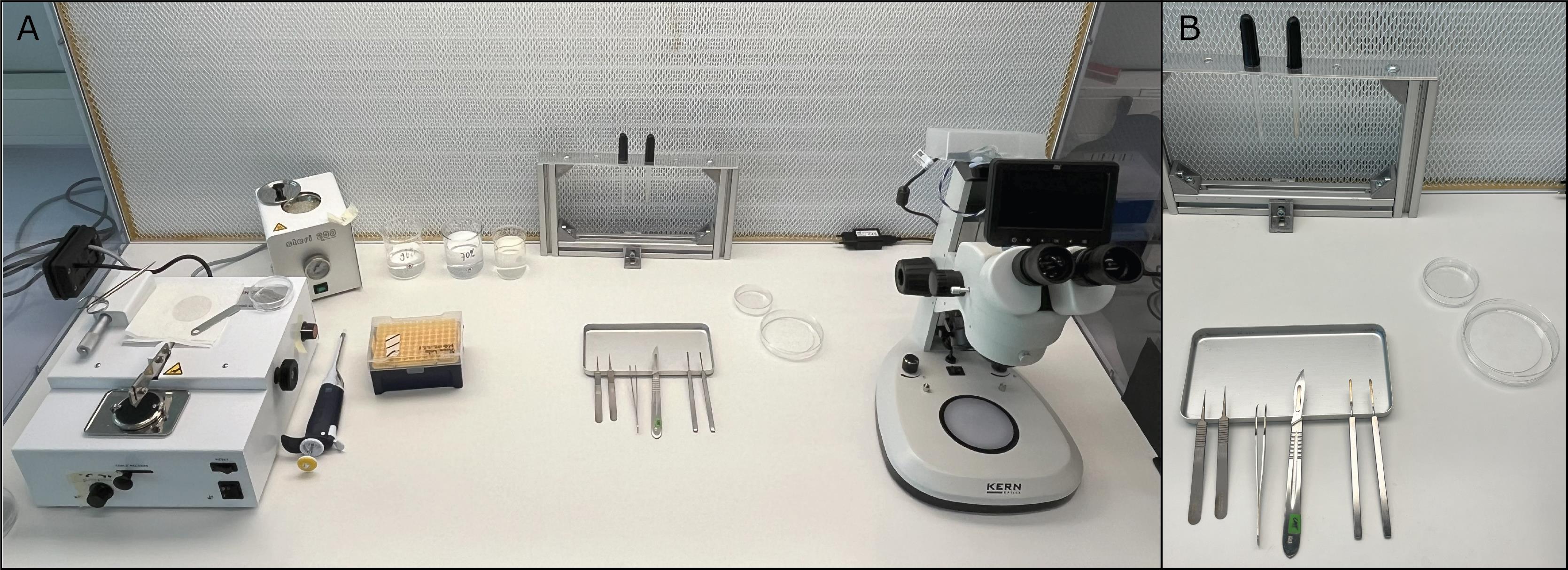
Figure 1. Dissection tools and working area. A. Overview of the working area and essential tools needed for dissection. From left to right: chopper, sterilizer, 200 μL pipette and tips, dissection tools, Petri dishes, and a microscope. B. Zoom-in view of essential dissection tools. From left to right: broken straight tweezers (two halves), bent tweezers, scalpel, two round spatula tools, and two glass pipettes in the rack smoothened using a Bunsen burner (one with a ~2 mm opening and one with a ~5 mm opening).
2. Decapitation and brain removal:
Note: Researchers should receive appropriate training before conducting decapitation and follow the local regulations of the animal welfare body regarding animal experiments.
a. Before decapitation, take out the 40 mL GBSS from the freezer and gently shake it, so it becomes “slushy”. Also, take out the 15 mL tube with GBSS from the fridge. Put both tubes on ice. Figure 2 shows the final setup of the decapitation area.
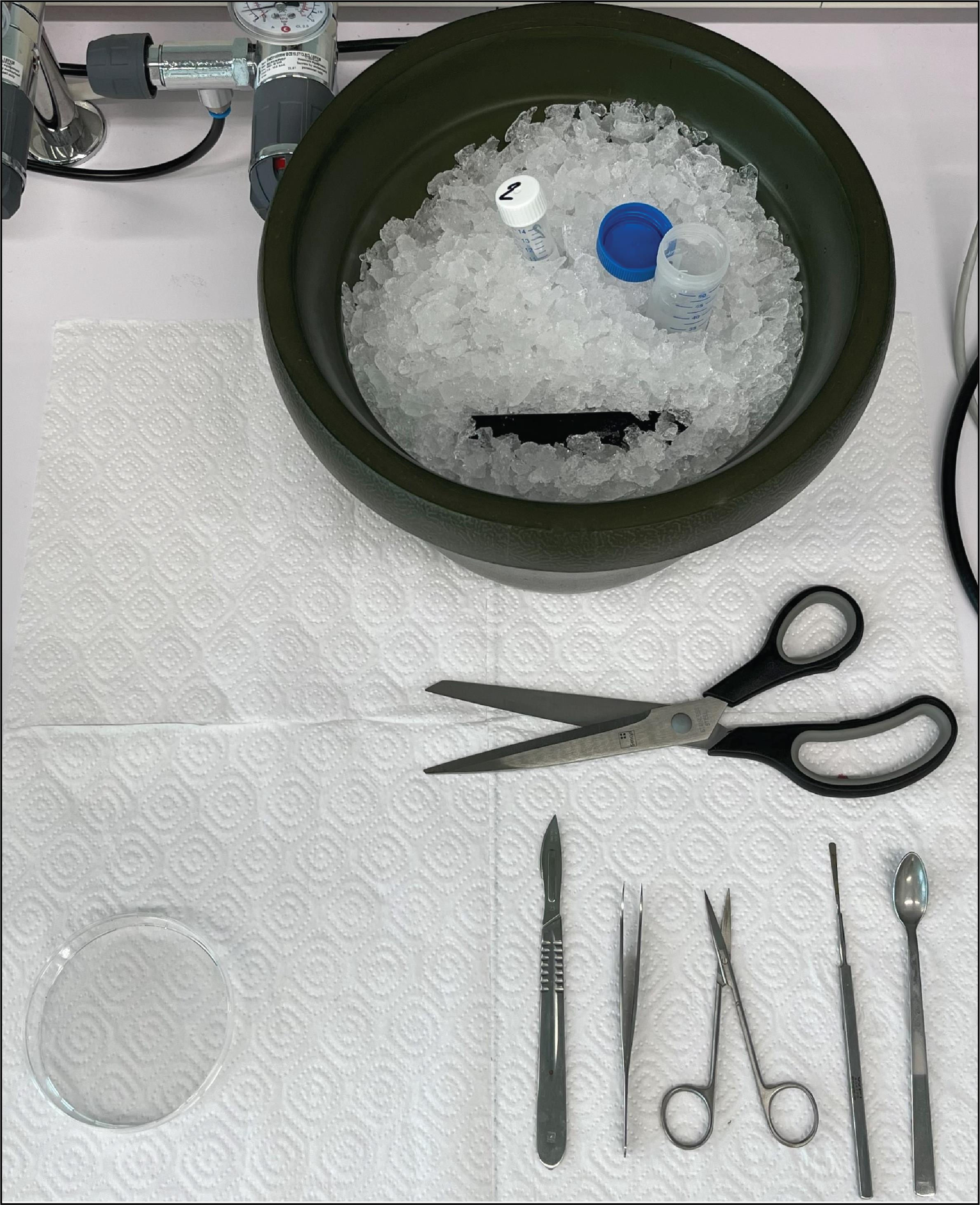
Figure 2. Decapitation tools and reagents. The blue-capped tube contains ~40 mL GBSS, which has been in the freezer for 45 min. The white-capped 15 mL tube contains cold GBSS from the fridge. The black metal plate is cooled in the ice bucket and is used during dissection to cool the Petri dish with GBSS. Brain dissection tools from left to right: scalpel, tweezers, scissors, spatula, and a small spoon. The big scissors are used for decapitation.
b. Take the mouse pup and quickly decapitate using a pair of sharp scissors.
Note: Cup your hands in order to calm the mouse pup before decapitation; make sure there is no ethanol on your gloves.
c. After decapitation using the big scissors, use the scalpel to cut the skin on top of the head open across the brain’s midline and fold it to the side/front with tweezers or your fingers.
d. Then, use the scissors to cut open the skull from posterior to anterior along the midline. Insert the scissors at lambda or from behind the cerebellum, pull upward slightly to prevent damage to the brain, and then cut the skull open in one go. Fold the skull to the side using tweezers.
e. Scoop out the brain using a spatula and put it into the “slushy” GBSS. Let it cool down for 1 min (while cleaning the dissection tools).
f. Pour all the GBSS into the big Petri dish with the filter paper and use the small spoon to transfer the brain.
Note: Filter paper helps with holding the brain in place whilst performing dissection.
3. Isolating the hippocampus:
a. First, cut off the anterior (olfactory bulb and part of the frontal cortex) and posterior (cerebellum) parts of the brain (Figure 3A).
b. Then, separate the two hemispheres by cutting across the midline (Figure 3B–3C).
c. Put the cold metal block underneath the Petri dish and proceed under the microscope.
d. Use the two round spatulas to carefully flip the brain on the anterior part with the cortex (round) side facing away from you. The midbrain is now visible (Figure 3D).
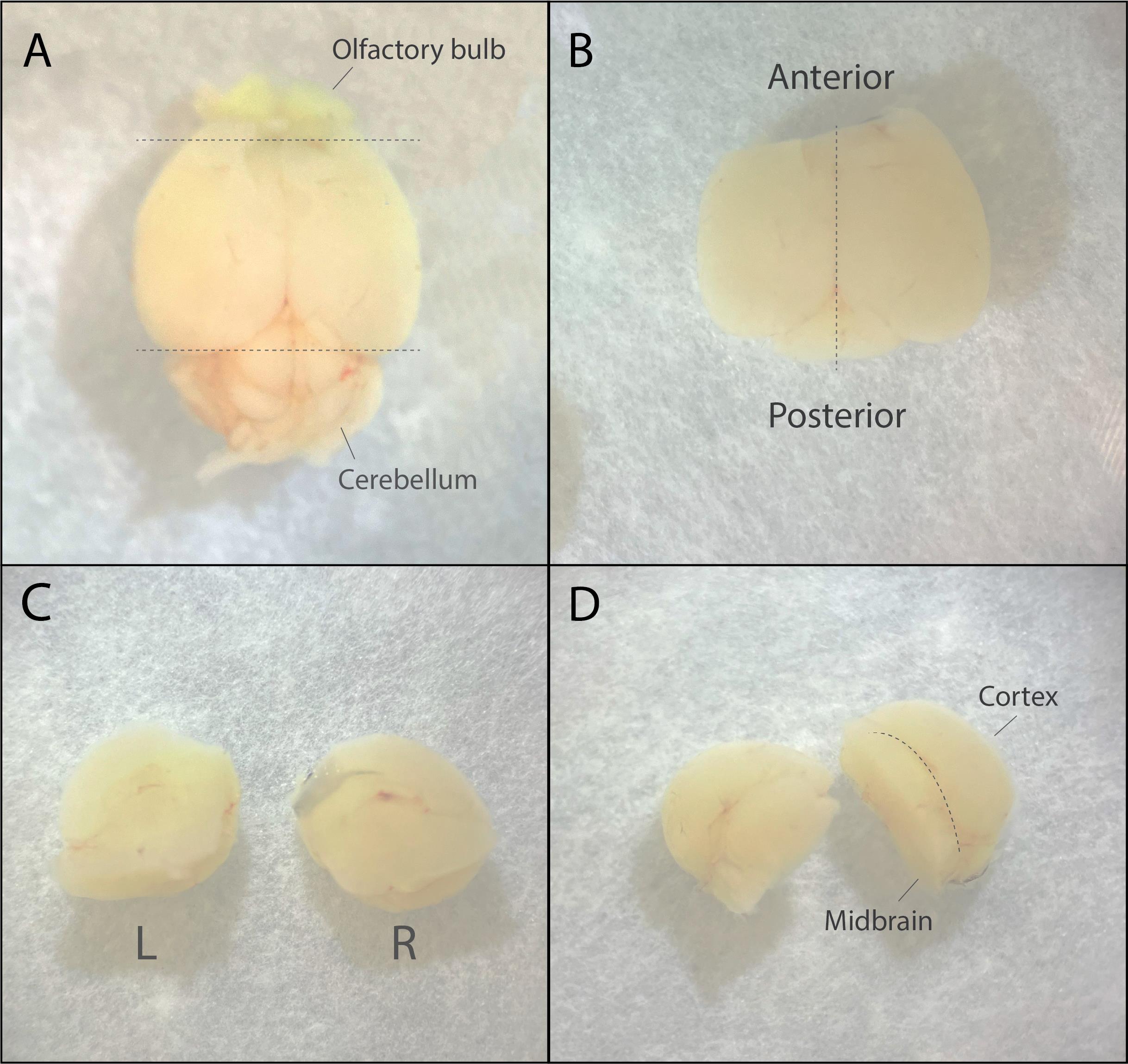
Figure 3. Dissection steps of the whole brain to separate hemispheres. A. Dorsal view of the brain. Dotted lines indicate the regions that need to be cut off. B. Dorsal view of the brain after cutting; the dotted line indicates the cut to separate the two hemispheres. C. Left and right hemispheres separated, viewing the midbrain. D. Put the hemispheres on the anterior part; the outside (round) part is the cortex, and the inside part is the midbrain.
e. Scoop out the midbrain: insert the spatula at the dotted line (Figure 3D) and scoop it out in one motion.
Note: If you are not able to scoop out the full midbrain, try to remove the rest with the spatula but prioritize not damaging the hippocampus.
f. Put the brain down on the cortex so that the hippocampus is facing you (Figure 4A). The hippocampus should now be visible as a banana-shaped structure lying on top of the cortex. Cut the left and right sides off so the hippocampus becomes separated from the cortex.
Note: Cutting more off the sides makes the hippocampus easier to roll out but reduces the yield of slices.
g. “Roll” the hippocampus out and over the cortex using two spatulas. Use one spatula to stabilize the cortex and the other to slide between the cortex and the hippocampus from the side. Flip the hippocampus out and away from you. The hippocampus is still attached to the cortex; cut it loose in one motion using the spatula. Do not cut the cortex too close to the hippocampus, making sure some of the entorhinal cortex is still attached. Perform steps A3d–f for both hippocampi.
Notes:
1. When the hippocampus is separated, some fibrous membranes may still be attached to it. Try to carefully remove these with the round side of the bent tweezer.
2. When you need to move the separated hippocampus, always use the glass pipette with the ~5 mm opening to avoid damage. If you have to touch it with tools, only touch the cortex side.
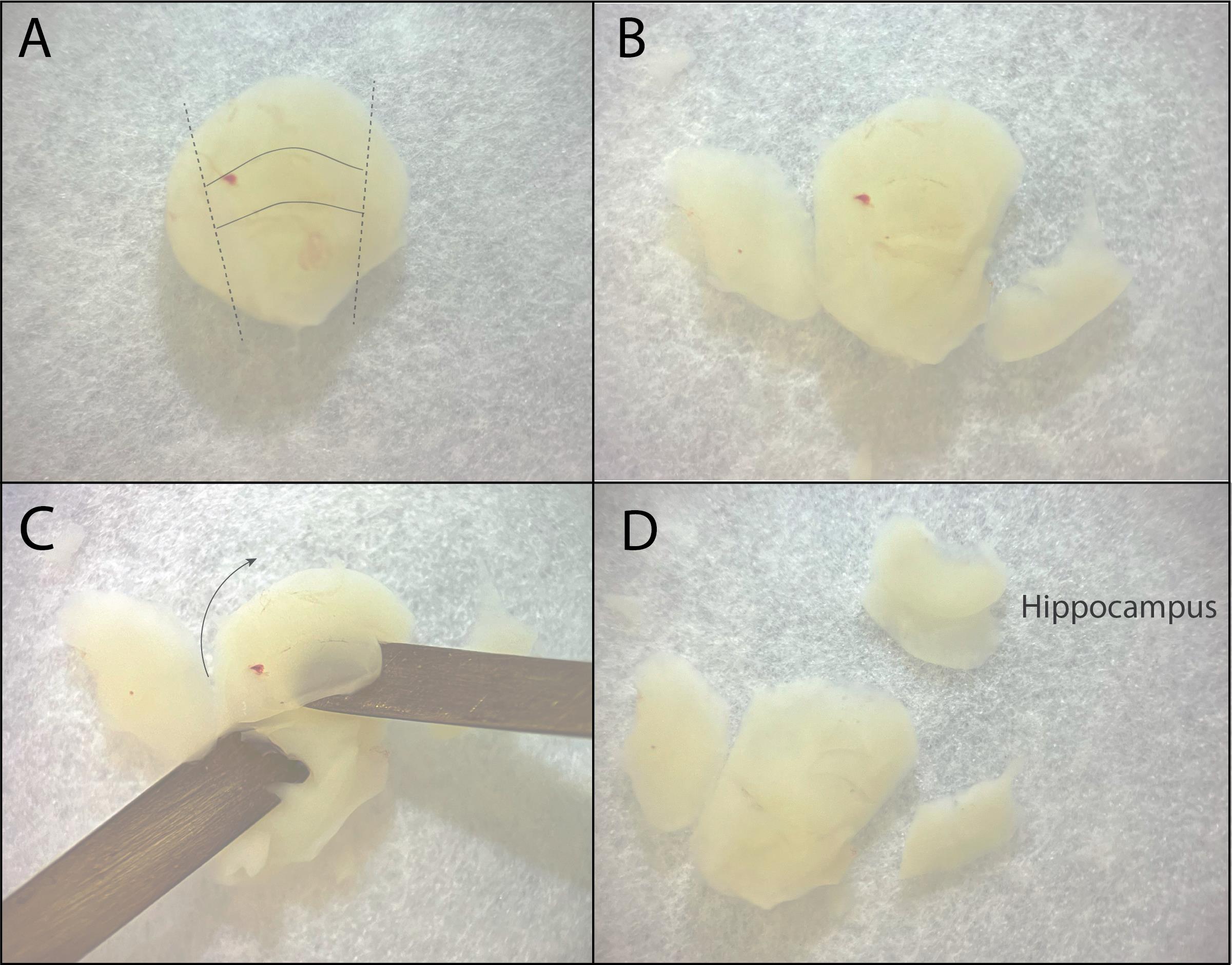
Figure 4. From hemisphere to hippocampus. A. The hippocampus is visible as a banana-shaped structure lying against the cortex. Dotted lines indicate where to cut to loosen the hippocampus. B. Hemisphere with hippocampus after cutting. C. Scoop out the hippocampus with the spatulas in one motion. D. View of the hippocampus after rolling it out, with a piece of entorhinal cortex still attached.
h. Now, put both hippocampi onto the PVC membrane using the glass pipette (Figure 5A). Align the two hippocampi parallel to each other and orthogonal to the razor blade. The thicker, round dorsal side of the hippocampus should preferably be closest to the razor blade so that it will be cut first. Remove any excess GBSS with a 200 μL pipette.
i. Use the chopper to make 400 μm vertical slices.
j. Fill the small Petri dish with 15 mL cold GBSS. Transfer the PVC membrane with the slices to the Petri dish. Use the tweezers to abruptly push the PVC into the cold GBSS fluid. This will prevent the hippocampal slices from detaching.
Note: Some slices may detach from the PVC. In this case, carefully get them to sink back to the bottom by gently dropping a droplet on top of them using the glass pipette with the ~2 mm opening.
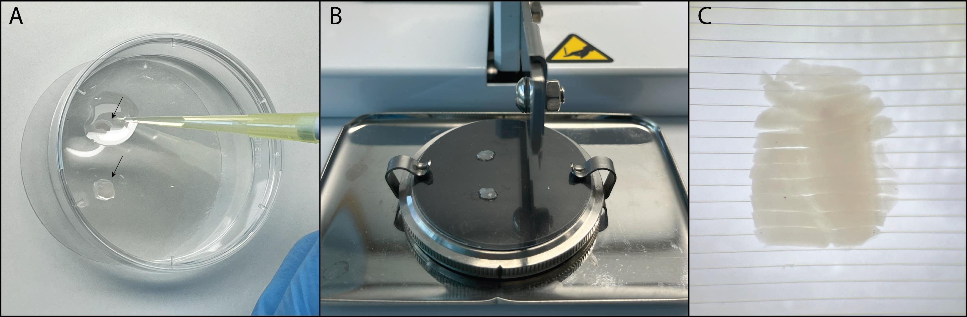
Figure 5. Making hippocampal slices using the tissue chopper. A. Put the hippocampus with the CA1 region facing upward onto the PVC membrane. Make sure the hippocampus is orthogonal to the razor blade. B. Place the PVC membrane on the chopper. C. View of hippocampal slices under the microscope after cutting on the chopper.
k. Separate the hippocampal slices (Figure 6A). Enter with one broken tweezer from the side of the entorhinal cortex and hold the slice in place at the hippocampal side; this way, our region of interest (CA1) is not damaged. Make sure to move your tools only in a horizontal direction to minimize touching the slices.
l. If a slice has a large entorhinal cortex, make sure to cut this a bit smaller (approximately 1/3 of the size of the hippocampal part; Figure 6B–6C). Slices with too much or too little entorhinal cortex are often of lower quality.
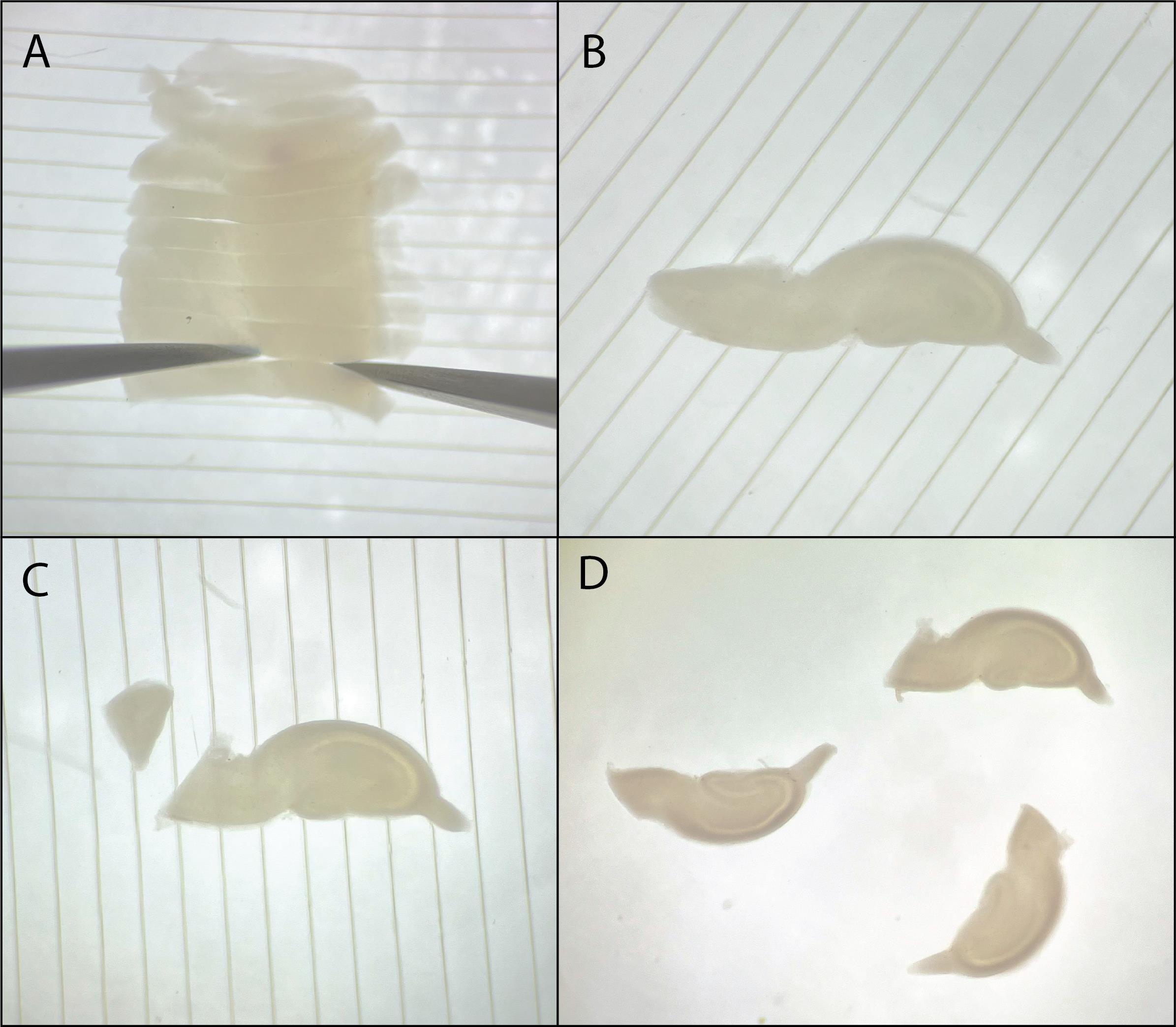
Figure 6. Separating and trimming hippocampal slices. A. Separate hippocampal slices using broken tweezer tools. B. Example of a good hippocampal slice before cutting the entorhinal cortex. C. Hippocampal slice after cutting the entorhinal cortex. D. Three good hippocampal slices with cut entorhinal cortices.
4. Plating and maintaining slices:
a. Select the best slices for culturing. Pick up one slice into the pipette and release it in a single droplet onto the PTFE membrane in the insert (Figure 7A–B). Take away excess fluid using a 200 μL pipette without touching the slice (Figure 7C).
Notes:
1. Sometimes, the slice will float toward the pipette tip when taking away excess fluid. Therefore, place the tip at the cortex side to prevent accidental damage to the CA1.
2. Plating the slices on small membrane cutouts allows easy transfer of the slices from the inserts to the microscope setup. Alternatively, the slices can be placed directly onto the inserts.
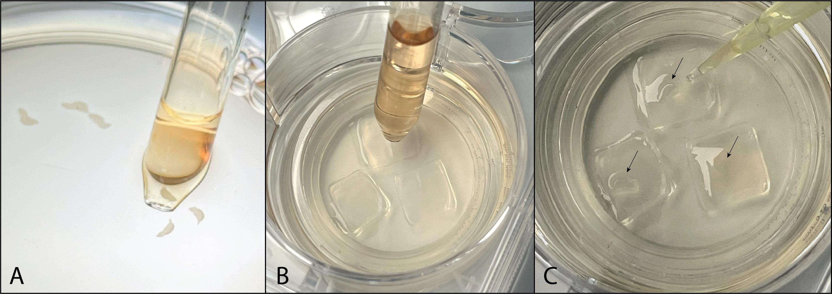
Figure 7. Plating hippocampal slices. A. Use a pipette to pick up a single hippocampal slice. B. Drop it directly in the middle of a PTFE membrane. C. Remove excess culture medium using a 200 μL pipette.
b. Refresh the culture medium the next day: take out the culture insert using sterilized tweezers in a closed flow hood. Aspirate the medium and add 1 mL of fresh culture medium with a sterilized pipette tip. Then, put the insert back into the well.
c. From then on, refresh the medium every other day.
Note: Refreshing 2 times per week is also sufficient. Slices can be kept in culture for ~4 weeks. Figure 8 shows a representative slice over time.
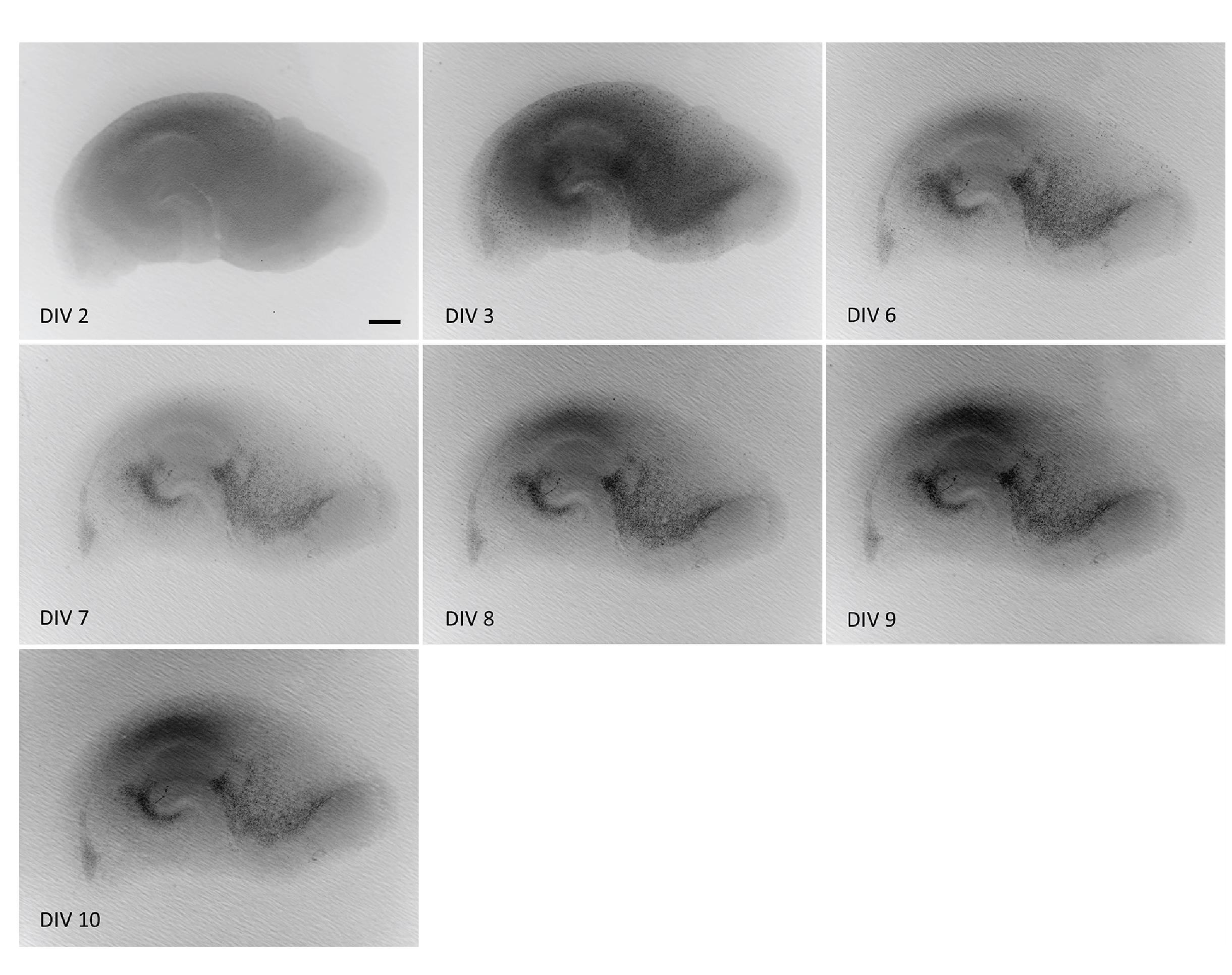
Figure 8. Representative images of a hippocampal slice on different days in vitro (DIV). Slices will look different over time. Right after dissection, hippocampal structures are well visible. As the slice flattens and attaches to the PTFE membrane, its appearance changes. The dark color disappears over time, as damaged cells are cleared, and the slice becomes thinner. Good-quality slices maintain a clear anatomical structure and stable thickness at ~150 μm after DIV10. Scale bar = 250 μm.
B. Determine optimal virus concentration
Notes:
1. Adeno-associated viruses (AAVs) were prepared in HEK293 cells [16]. For more details on the SClm viruses, we refer readers to Grimley et al. [11] and Peerboom et al. [17].
2. Alternatively, slices can be prepared from transgenic mice in which SClm is expressed in (a subset of) neurons [14]. This alleviates the need for AAV-mediated transduction.
1. Prepare a range of viral concentrations.
a. Dilute the virus in PBS, ensuring that it is kept on ice. Testing a range of viral concentrations is advised. We tested undiluted (titer of 1.12 × 10¹² genomic copies per milliliter), 1:2, 1:5, 1:10, 1:25, and 1:50 virus dilutions.
Note: The dilution factor that is used depends not only on viral titer but also on the type of construct (floxed vs. non-floxed). Therefore, we advise always using a dilution range to determine the concentration that gives optimal expression of the SClm sensor.
2. Inject the virus into the CA1 region of the hippocampus.
a. Before performing AAV-mediated transduction, refresh with 1 mL of culture medium.
b. After pulling a thin-walled glass capillary in a pipette puller, secure it in the micromanipulator holder.
c. Before adding the virus to the pipette, cut the tip of the glass pipette using a small pair of scissors under a wide-field microscope. See Figure 9 for the approximate size of the pipette tip opening.
Note: Keep the magnification you use (we use 32× magnification) consistent when cutting the pipette tip to minimize the variation of pipette tip openings.
d. Ensure that the microinjector is turned on. Set the injection pressure to ~80 hPa.
Note: The exact pressure strength will need to be tuned, as this parameter is also dependent on the size of the capillary opening.
e. Take the capillary from its holder and add the virus to the capillary using a 20 μL pipette with a microloader pipette tip. Attach the filled capillary back to the holder.
f. Move the capillary toward the slice. Make sure to position the capillary above the slice between the CA1 and the Dentate gyrus when targeting VGAT-Cre cells in the stratum radiatum. When targeting pyramidal cells, injections (of Cre-independent virus) should be performed close to but not in the stratum pyramidale.
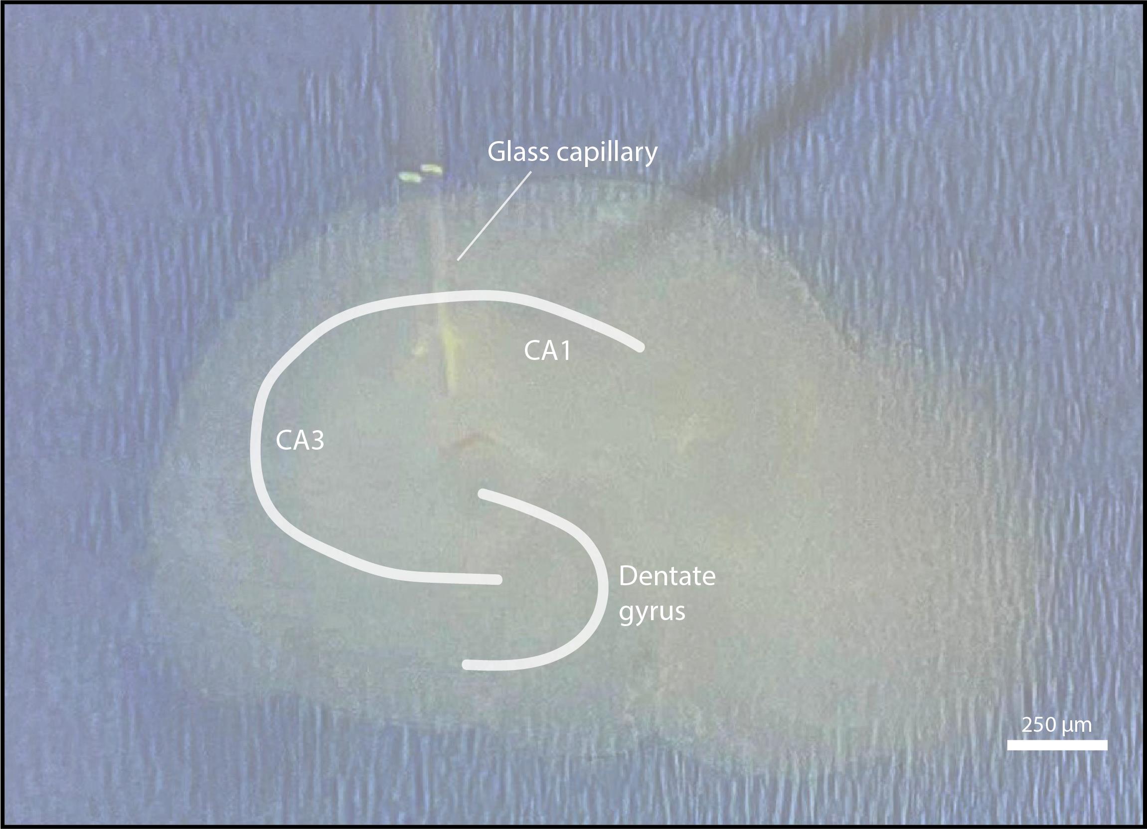
Figure 9. AAV injections in organotypic hippocampal slices. The glass capillary is placed between the CA1 region and the dentate gyrus. After applying pressure, a droplet containing virus will form in the middle of the slice. Scale bar = 250 μm.
g. Move the capillary toward the slice until it touches the surface of the slice. You can now inject. A bubble will form on top of the slice. Make sure that the bubble is not too big and that it does not roll off the slice for optimal transfection. Injecting slightly below the cell surface will result in more localized expression. We typically inject at 3–4 locations for optimal results.
C. SClm sensor calibration (slightly modified from Grimley et al. [11])
Note: The FRET ratio is dependent on the type of microscope used, its settings, and its filters. Therefore, it is essential that the calibration and imaging of experiments are performed on the same microscope using the same filters and settings.
1. Prepare chloride stocks.
a. Prepare high chloride stock, low chloride stock, and KF quenching solution (see Recipes).
b. Use the high and low chloride stock to make dilutions containing 0 mM (0 mL of high and 100 mL of low chloride stock), 5 mM (8 mL of high and 92 mL of low chloride stock), 10 mM (16 mL of high and 84 mL of low chloride stock), 50 mM (32 mL of high and 68 mL of low chloride stock), and 161 mM (100 mL of high and 0 mL of low chloride stock) of chloride. Adjust pH to 7.4 if necessary, using NaOH or HCl.
2. Measure SClm FRET signals using ionophore treatment.
a. Wash in aCSF containing ionophores (100 μM nigericin and 50 μM tributyltin acetate) at a flow rate of 1 mL/min for 20 min.
b. Perfuse slices with saline solutions containing 0, 5, 10, 50, and 161 mM of chloride and the ionophores in the abovementioned concentration. Finish by washing in the KF quenching solution (+ ionophores) to maximally quench the SClm sensor.
c. Consequently perfuse slices with these solutions, 15 min per solution. Take a Z-stack image every 5 min (see section D).
Notes:
1. We experienced highly variable penetrance of nigericin and tributyltin in organotypic hippocampal slices between experiments, probably due to the high cell density and thickness. It is therefore important to monitor SClm responses and make sure FRET signals are stable and reflect equal intra- and extracellular chloride concentration. The FRET ratios in the plateau phase (usually reached after ~10 min) should be used for creating the calibration curve. If possible, perform calibration in dissociated cultures, where ionophores have more direct access to the cells.
2. Slice quality will decrease during ionophore treatment; usually, only 3 or 4 concentrations can be tested per slice.
D. Imaging
1. Make ACSF solution (see Recipes) and measure the pH (7.2–7.4) and osmolarity (310 ± 10 mOsmol/L).
2. Perfuse the bath of the two-photon microscope system with 1 mL/min of ACSF heated to 30–32 °C and continuously carbonated (start carbonation 20–30 min before the experiment) with 5% CO2 and 95% O2.
3. Transfer a slice into the bath with the CA1 region of the hippocampus facing away from you.
4. Locate the stratum pyramidale of the CA1 region of the hippocampus using a 4× objective and zoom in using a 60× water immersion objective.
5. Find cells with good SClm sensor expression. Determine appropriate laser power based on expression levels to minimize bleaching.
6. Image Z-stacks in multiple fields of view (FOVs) in the stratum pyramidale (when imaging pyramidal cells) or the stratum radiatum (when imaging inhibitory interneurons). We usually image 2–4 FOVs per slice.
Note: We mainly acquire image stacks at a resolution of 8.1 pixels/μm (1,024 × 1,024 pixels, 126 × 126 μm) with 1-μm steps of ∼40–85 μm in depth. If your experiment requires frequent imaging (e.g., every 2 min), the resolution should be decreased (e.g., 4.1 pixels/μm, 512 × 512 pixels, 126 × 126 μm) to shorten the image acquisition time.
Data analysis
A. Image analysis in ImageJ/Fiji
1. Drawing regions of interest (ROIs) and calculating FRET ratios.
a. Install the ImageJ/Fiji macro MacroRG_final.
b. Open the donor (CFP) and the corresponding acceptor (YFP) stacks.
c. Zoom in on the cell of interest using the magnifying glass. Use freehand selection to draw a ROI around the cell.
Notes:
1. Only use cells that are within 450 pixels of the center. Cells in the perimeter of the FOV could give inaccurate FRET ratios.
2. Try to select cells with varied brightness (bright, middle, and dark) to get a representative dataset.
d. Press T to save the ROI to the ROI manager.
e. Repeat steps A1a–d for two other cells in the FOV. Only select cells in the same z-plane.
f. When finished, also draw a ROI for the background.
g. Press F to run MacroRG_final.
h. Save the folder with ROI results. Make a separate folder per time point.
i. The script automatically subtracts the CFP and YFP background intensity (step A1f) from the CFP and YFP channel intensities. The output is saved in an Excel file.
j. The script automatically divides the YFP intensity by the CFP intensity to obtain the FRET ratio. This output is saved in an Excel file.
k. Repeat steps A1c–j for cells in other z-planes and/or for each imaging time point.
l. Create a calibration curve by plotting the measured FRET ratios for each chloride concentration. Fit with the calibration equation to obtain the relation between FRET ratio and chloride concentrations for all subsequent measurements [11,15]:
Where R represents the YFP/CFP emission ratio, Kd represents the dissociation constant, and Rmin and Rmax represent the minimum and maximum FRET ratios, respectively.
Notes:
1. As discussed previously [15], converting FRET signals into chloride concentration is not always needed. In many cases, FRET ratios can be compared between cells in the same image or between multiple time points within one experiment. In those cases, it may be preferred to report measured differences in FRET ratios directly.
2. It is important to understand that SClm FRET ratios also depend on intracellular pH. If you suspect there are pH changes in your experiments, there are good chloride sensors available that can also be used to measure pH [8].
B. Creating FRET-colored images (for illustration purposes only)
1. Calculating FRET ratios:
Note: Make FRET images for a small sub-stack that contains your cell(s) of interest, so that the FRET values are not altered by signals coming from cells in other Z planes.
a. Open the donor (CFP) and the corresponding acceptor (YFP) .tif image stacks and perform background correction by drawing a ROI in a central area without cells and measuring the average background pixel intensities for the CFP and YFP channels (Analyze > Measure).
b. Subtract the mean background values (Process > Math > Subtract) from the respective CFP and YFP image stack intensities.
Note: It is optional to median filter this image (Process > Filters > Median) at ~2 pixels to get rid of background noise. Before continuing, make sure to set the division by zero to 0 (Edit > Options >Misc, Divide by zero value: 0.0).
c. Smoothen images by applying a 3D Gaussian blur to CFP and YFP channels (Process > Filter > Gaussian Blur 3D). Choose sigma values that take into account the microscope resolution and step size in Z.
d. Before continuing, make sure to set the division by zero to 0.0 (Edit > Options > Misc, Divide by zero value: 0.0).
e. To make a ratiometric image, perform pixel-wise division of the acceptor (CFP) and donor (YFP) channels (Process > Image Calculator, CFP/YFP). Select 32-bit (float) Result.
Note: From our experience, we found that FRET ratios lower than 0.5 or higher than 1.6 usually represent unhealthy cells. However, these FRET values depend on the settings of the microscope and its filters.
2. Generating masks:
Option 1, automatic mask generation (see Figure 10C):
a. Perform pixel-wise multiplication of the acceptor (CFP) and donor (YFP) channels (Process > Image Calculator).
b. Threshold the result (Image > Adjust > Threshold) to the corresponding level of the product of the average background intensities of both channels as calculated in step B1b (e.g., YFP background = 100, CFP background = 105, so 100 * 105 = threshold to 10,500). Select the option “set background pixels to NaN” and press No to not process all images. This procedure selects pixels that show high intensity in both CFP and YFP channels.
c. Convert to mask (Process > Binary > Convert to mask). Deselect “calculate threshold for each image” and “only convert current image” and select “black background/list thresholds” (Figure 10C).
Note: It is optional to median filter this image (Process > Filters > Median) ~5 pixels to get rid of small puncta.
Option 2, manual mask selection (see Figure 10F):
d. Make a max projection of a specific range from the acceptor (CFP) Z-stack. Manually draw ROIs around cells of interest and press delete.
e. To use these ROIs as the mask, click Process > Math > Max and set Value = 1.
f. Adjust > Threshold to switch to black and white (B&W).
g. Now, generate the mask (Process > Binary > Convert to mask).
3. Generating a projection and applying the masks to create a FRET-colored image:
a. Find a Z-range with a number of cells with good SClm sensor expression to make a projection of.
b. Produce an average (!) Z-stack projection (Image > Stacks > Z project) for the ratiometric image obtained in B1d (Figure 10A) and a maximum projection (!) for the donor channel (YFP) from step B1d (Figure 10B) and the mask from step B2c or g (Figure 10C).
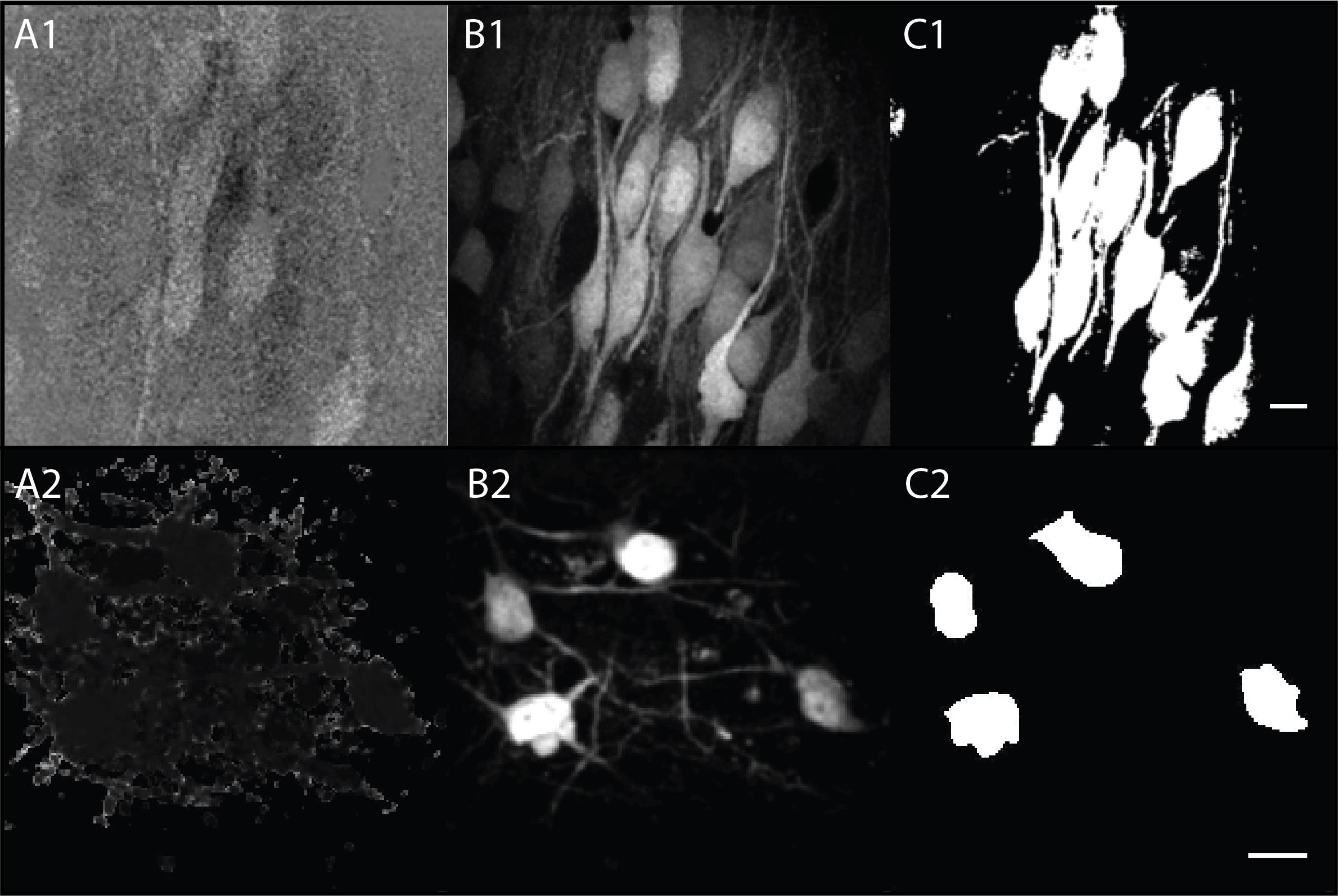
Figure 10. Different Z-projections needed for creating ratiometric masks. (A1, B1, C1) Examples of pyramidal cells. (A2, B2, C2) Examples of interneurons. (A) Average Z-stack of ratiometric images obtained in step B1d. (B) Maximum projection of donor channel (YFP) from step B1d. (C) Maximum projection of mask from step B2 using automatic masking. Scale bars = 20 μm.
c. Convert the maximum projection binary mask value from 255 to 1 using Process > Math > Max, set Value = 1.
Note: The image turns black.
d. Multiply the averaged ratiometric image from step B3b (Figure 10A) with the maximum binary mask from step B3c (background:0, signal:1) (Process > Image Calculator). You now have an image that only shows the ratiometric image within the mask.
e. Select the masked ratiometric image from step B3d and import the custom categorical look-up table (LUT) (File > Import > LUT) “FRET_categorical_8_color_v3.lut”. This will automatically apply the LUT to the image (Figure 11A). Use Image > Adjust > Brightness/Contrast to set the proper range to only include healthy cells (this is dependent on the microscope setup; we used min = 0.4 and max = 1.5).
f. Duplicate the binary mask from step B2c or B2g, invert the values (Edit > Invert), and subtract 254 from the image (Process > Math > Subtract). This provides you with the inverse mask of step B2c or g.
g. Multiply the maximum Z-projection of the donor channel (YFP) from step B3b (Figure 10B) with the duplicated inverted mask from step B3f (Process > Image Calculator). Now, all the pixels used for the ratiometric image appear in black in the grayscale image of the donor channel (Figure 11B).
h. Combine the ratiometric image from step B3e and the grayscale image from step B3g (Image > Color > Merge Channels) and select “Create composite” and “Keep source images” since the LUT may need to be readjusted for both images. Open the LUT table with Analyze > Tools > Calibration bar and adjust the LUT if needed (Figure 11C).
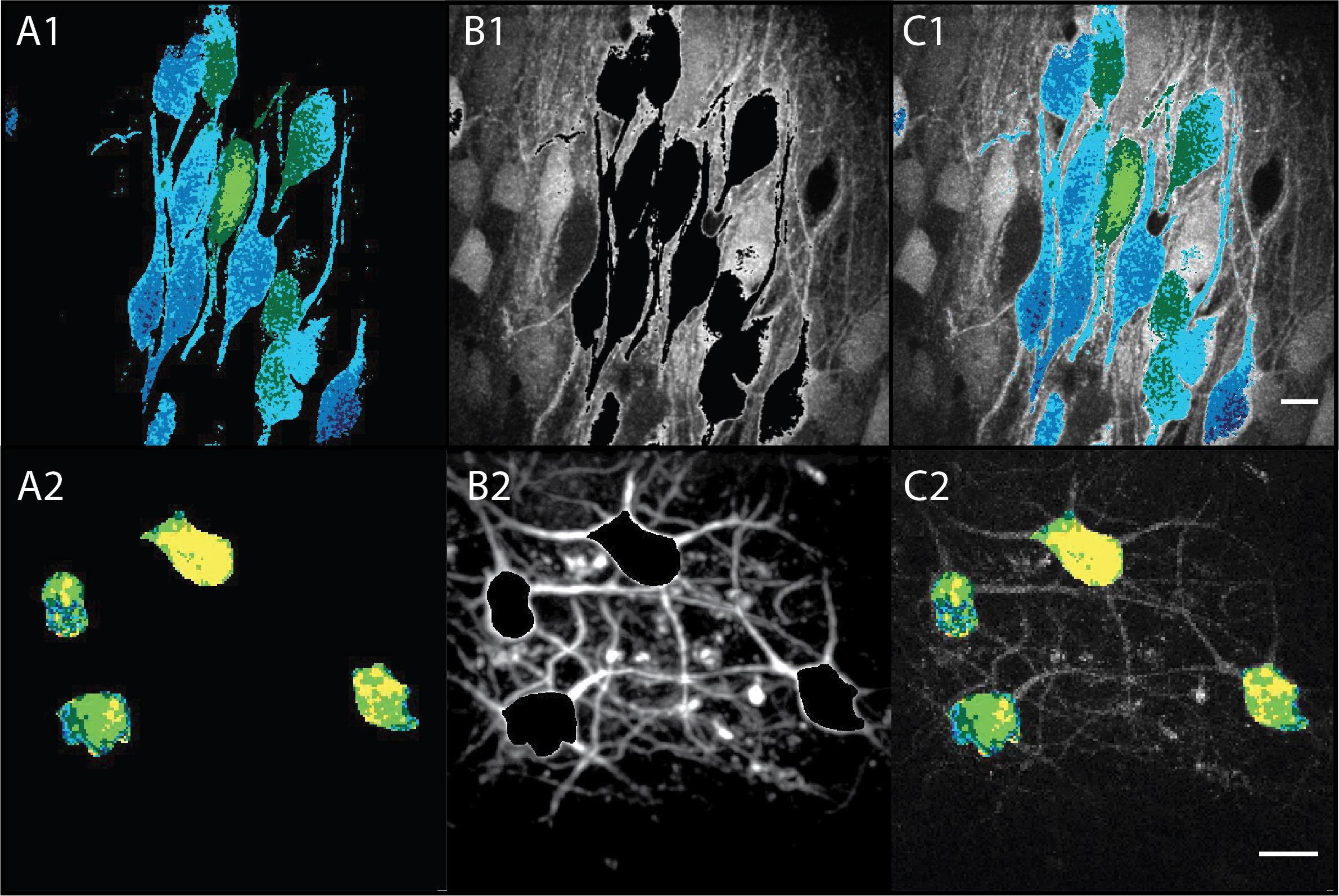
Figure 11. Applying the ratiometric mask to create illustrative images displaying the FRET ratio. (A1, B1, C1) Examples of pyramidal cells. (A2, B2, C2) Examples of interneurons. (A) Mask showing the FRET ratio indicated by color. Yellow = low FRET ratio; blue = high FRET ratio. (B) Maximum projection of the donor channel (YFP) with an automated mask overlay (step B3g). (C) Ratiometric overlay created by merging A and B. Scale bars = 20 µm.
Validation of protocol
The protocol described in this paper was used and validated in the following two papers published by our lab:
Herstel et al. [15]. Using SuperClomeleon to Measure Changes in Intracellular Chloride during Development and after Early Life Stress. eNeuro.
Peerboom et al. [17]. Delaying the GABA Shift Indirectly Affects Membrane Properties in the Developing Hippocampus. J Neurosci.
Acknowledgments
This work was supported by the NWO grants NWA.1518.22.136 SCANNER and OCENW.KLEIN.150.
We would like to thank Prof. Kevin Staley for providing the non-floxed SClm virus and Prof. Thomas Kuner for providing the floxed SClm construct. We would like to thank René van Dorland and Dr. Eric Jansen for their excellent technical support and virus production.
Competing interests
The authors declare no competing financial interests.
References
- Ben-Ari, Y. (2002). Excitatory actions of gaba during development: the nature of the nurture. Nat Rev Neurosci. 3(9): 728–739. https://doi.org/10.1038/nrn920
- Peerboom, C. and Wierenga, C. J. (2021). The postnatal GABA shift: A developmental perspective. Neurosci. Biobehav. Rev. 124: 179–192. https://doi.org/10.1016/j.neubiorev.2021.01.024
- Wang, D. D. and Kriegstein, A. R. (2010). Blocking Early GABA Depolarization with Bumetanide Results in Permanent Alterations in Cortical Circuits and Sensorimotor Gating Deficits. Cereb Cortex. 21(3): 574–587. https://doi.org/10.1093/cercor/bhq124
- Hui, K. K., Chater, T. E., Goda, Y. and Tanaka, M. (2022). How Staying Negative Is Good for the (Adult) Brain: Maintaining Chloride Homeostasis and the GABA-Shift in Neurological Disorders. Front Mol Neurosci. 15: e893111. https://doi.org/10.3389/fnmol.2022.893111
- van van Hugte, E. J. H., Schubert, D. and Nadif Kasri, N. (2023). Excitatory/inhibitory balance in epilepsies and neurodevelopmental disorders: Depolarizing γ‐aminobutyric acid as a common mechanism. Epilepsia. 64(8): 1975–1990. https://doi.org/10.1111/epi.17651
- Tyzio, R., Holmes, G. L., Ben‐Ari, Y. and Khazipov, R. (2007). Timing of the Developmental Switch in GABAA Mediated Signaling from Excitation to Inhibition in CA3 Rat Hippocampus Using Gramicidin Perforated Patch and Extracellular Recordings. Epilepsia. 48: 96–105. https://doi.org/10.1111/j.1528-1167.2007.01295.x
- Hess, S., Wratil, H. and Kloppenburg, P. (2023). Perforated Patch Clamp Recordings in ex vivo Brain Slices from Adult Mice. Bio Protoc. 13(16): e4741. https://doi.org/10.21769/bioprotoc.4741
- Lodovichi, C., Ratto, G. M., Trevelyan, A. J. and Arosio, D. (2022). Genetically encoded sensors for Chloride concentration. J Neurosci Methods. 368: 109455. https://doi.org/10.1016/j.jneumeth.2021.109455
- Arosio, D. and Ratto, G. M. (2014). Twenty years of fluorescence imaging of intracellular chloride. Front Cell Neurosci. 8: 258. https://doi.org/10.3389/fncel.2014.00258
- Kuner, T. and Augustine, G. J. (2000). A Genetically Encoded Ratiometric Indicator for Chloride. Neuron. 27(3): 447–459. https://doi.org/10.1016/s0896-6273(00)00056-8
- Grimley, J. S., Li, L., Wang, W., Wen, L., Beese, L. S., Hellinga, H. W. and Augustine, G. J. (2013). Visualization of Synaptic Inhibition with an Optogenetic Sensor Developed by Cell-Free Protein Engineering Automation. J Neurosci. 33(41): 16297–16309. https://doi.org/10.1523/jneurosci.4616-11.2013
- Côme, E., Blachier, S., Gouhier, J., Russeau, M. and Lévi, S. (2023). Lateral Diffusion of NKCC1 Contributes to Chloride Homeostasis in Neurons and Is Rapidly Regulated by the WNK Signaling Pathway. Cells. 12(3): 464. https://doi.org/10.3390/cells12030464
- Boffi, J. C., Knabbe, J., Kaiser, M. and Kuner, T. (2018). KCC2-dependent Steady-state Intracellular Chloride Concentration and pH in Cortical Layer 2/3 Neurons of Anesthetized and Awake Mice. Front Cell Neurosci. 12: e00007. https://doi.org/10.3389/fncel.2018.00007
- Rahmati, N., Normoyle, K. P., Glykys, J., Dzhala, V. I., Lillis, K. P., Kahle, K. T., Raiyyani, R., Jacob, T. and Staley, K. J. (2021). Unique Actions of GABA Arising from Cytoplasmic Chloride Microdomains. J Neurosci. 41(23): 4957–4975. https://doi.org/10.1523/jneurosci.3175-20.2021
- Herstel, L. J., Peerboom, C., Uijtewaal, S., Selemangel, D., Karst, H. and Wierenga, C. J. (2022). Using SuperClomeleon to Measure Changes in Intracellular Chloride during Development and after Early Life Stress. eNeuro. 9(6): ENEURO.0416–22.2022. https://doi.org/10.1523/eneuro.0416-22.2022
- McClure, C., Cole, K. L. H., Wulff, P., Klugmann, M. and Murray, A. J. (2011). Production and Titering of Recombinant Adeno-associated Viral Vectors. J Visualized Exp. 57: e3791/3348–v. https://doi.org/10.3791/3348-v
- Peerboom, C., de Kater, S., Jonker, N., Rieter, M. P., Wijne, T. and Wierenga, C. J. (2023). Delaying the GABA Shift Indirectly Affects Membrane Properties in the Developing Hippocampus. J Neurosci. 43(30): 5483–5500. https://doi.org/10.1523/jneurosci.0251-23.2023
Article Information
Publication history
Received: Nov 26, 2024
Accepted: Jan 26, 2025
Available online: Feb 25, 2025
Published: Mar 5, 2025
Copyright
© 2025 The Author(s); This is an open access article under the CC BY-NC license (https://creativecommons.org/licenses/by-nc/4.0/).
How to cite
Readers should cite both the Bio-protocol article and the original research article where this protocol was used:
- de Kater, S., Herstel, L. J. and Wierenga, C. J. (2025). Monitoring Changes in Intracellular Chloride Levels Using the FRET-Based SuperClomeleon Sensor in Organotypic Hippocampal Slices. Bio-protocol 15(5): e5229. DOI: 10.21769/BioProtoc.5229.
- Herstel, L. J., Peerboom, C., Uijtewaal, S., Selemangel, D., Karst, H. and Wierenga, C. J. (2022). Using SuperClomeleon to Measure Changes in Intracellular Chloride during Development and after Early Life Stress. eNeuro. 9(6): ENEURO.0416–22.2022. https://doi.org/10.1523/eneuro.0416-22.2022
Category
Neuroscience > Cellular mechanisms
Cell Biology > Cell imaging > Two-photon microscopy
Biophysics > Microscopy > Two-photon laser scanning microscopy
Do you have any questions about this protocol?
Post your question to gather feedback from the community. We will also invite the authors of this article to respond.