- Protocols

- Articles and Issues
- For Authors
- About
- Become a Reviewer

Quantifying Bacterial Chemotaxis in Controlled and Stationary Chemical Gradients With a Microfluidic Device


Published: Vol 15, Iss 4, Feb 20, 2025 DOI: 10.21769/BioProtoc.5184 Views: 1759
Reviewed by: Hsih-Yin TanAnonymous reviewer(s)
Advertisement


Protocol Collections
Comprehensive collections of detailed, peer-reviewed protocols focusing on specific topics


Related protocols
Abstract
Chemotaxis refers to the ability of organisms to detect chemical gradients and bias their motion accordingly. Quantifying this bias is critical for many applications and requires a device that can generate and maintain a constant concentration field over a long period allowing for the observation of bacterial responses. In 2010, a method was introduced that combines microfluidics and hydrogel to facilitate the diffusion of chemical species and to set a linear gradient in a bacterial suspension in the absence of liquid flow. The device consists of three closely parallel channels, with the two outermost channels containing chemical species at varying concentrations, forming a uniform, stationary, and controlled gradient between them. Bacteria positioned in the central channel respond to this gradient by accumulating toward the high chemoattractant concentrations. Video-imaging of bacteria in fluorescent microscopy followed by trajectory analysis provide access to the key diffusive and chemotactic parameters of motility for the studied bacterial species. This technique offers a significant advantage over other microfluidic techniques as it enables observations in a stationary gradient. Here, we outline a modified and improved protocol that allows for the renewal of the bacterial population, modification of the chemical environment, and the performance of new measurements using the same chip. To demonstrate its efficacy, the protocol was used to measure the response of a strain of Escherichia coli to gradients of α-methyl-aspartate across the entire response range of the bacteria and for different gradients.
Key features
• The protocol is based on a previously proposed system [1] that we improved for higher throughput.
• Setup allowing a rapid quantification of motility and chemotaxis responses.
• Seventeen hours were required from the start of an E. coli culture to the measurements to obtain the chemotactic velocity under various chemical conditions.
Keywords: MicrofluidicsGraphical overview
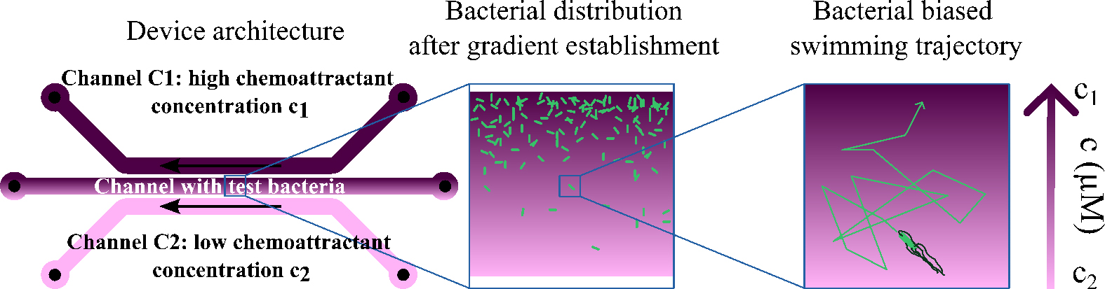
Schematic illustration of the three-channels chip architecture and its use with bacteria
Background
Bacterial chemotaxis is an important area of research that spans multiple fields. Examples include (i) microbiology, in which it helps to explain fundamental aspects of bacterial behavior, signaling pathways, and cellular processes; (ii) infectious diseases, where insights into how pathogenic bacteria use chemotaxis to locate and infect host tissues can inform the development of new treatments and preventive measures; (iii) environmental microbiology, in which chemotaxis is crucial for bacterial movement in natural environments, influencing nutrient cycling, bioremediation, and the functioning of microbial ecosystems; (iv) ecology and evolution, in which chemotaxis affects microbial interactions, competition, and cooperation within communities, providing insights into microbial ecology and the evolutionary dynamics of these behaviors; and (v) agriculture, where understanding how soil bacteria use chemotaxis to interact with plant roots can improve agricultural practices, enhance crop growth, and lead to the development of biofertilizers or biopesticides.
It is accepted that the chemotactic drift takes place at a velocity dependent on the detected concentration c and local gradient of the chemoattractant according to the following equation [2,3]:
(1)
where is the chemotactic susceptibility that depends on the local concentration
To this end, our microfluidic device uses diffusion through agar to generate a stable and controlled concentration and gradient and allows measuring precisely the vc for this environment. In practice, the gradient is established between parallel channels separated by a distance L, each containing a concentration cmin and cmax. Its value is and the average concentration of chemoattractant in which the bacteria swim is . Bacteria are introduced into the device, and their movement in response to the gradient is observed using microscopy. Bacteria swim toward the chemoattractant and gather on the channel wall closest to the source of the chemoattractant. Once the stationary regime is reached, the concentration of bacteria in this region decays exponentially, with a decay length:
(2)
This results from the competition between the advection of bacteria toward the source of chemoattractant at velocity vc and their active diffusion, which is characterized by a diffusion coefficient D. Here, the diffusion coefficient D is obtained by analyzing bacterial trajectories. This method enables the quantitative determination of chemotactic velocity and its dependence on the average concentration and its gradient. The chemotactic coefficient can be determined from the relation (see Eq. 1):
(3)
In its initial version, published by Ahmed et al. [1], the test required one microfluidic device per trial, making the method very time-consuming. Our protocol allows multiple trials to be run on the same chip, which may allow the method to be automated and enable continuous measurements. The method requires specialized equipment and expertise, which are presented here in detail. We illustrate the protocol using an Escherichia coli strain placed in α-methyl-aspartate gradients.
Materials and reagents
Biological materials
1. E. coli RP437 [7] (CGSC: #12122 transformed with the plasmid pZA3R-YFP carrying a chloramphenicol resistance marker and a yfp gene) stored in 25% glycerol in a -80 °C freezer for long-term conservation
Reagents
1. M9 salts (MP Biomedicals, catalog number: SKU 113037012-CF), dissolved in water at 22% (11 g in 50 mL)
2. Casamino acids (VWR, catalog number: ICNA113060012), dissolved in water at 5% (2.5 g in 50 mL)
3. D-(+)-Glucose (Sigma-Aldrich, catalog number: G7021-1KG), dissolved in water at 20% (10 g in 50 mL)
4. MgSO4·7H2O (Sigma-Aldrich, catalog number: 63138-250G), dissolved in water at 1 M (1.2 g in 50 mL)
5. KH2PO4 (Sigma-Aldrich, catalog number: P5655-500G), dissolved in water at 1 M (3.4 g in 25 mL water)
6. K2HPO4 (Sigma-Aldrich, catalog number: P3786-500G), dissolved in water at 1 M (4.3 g in 25 mL water)
7. CaCl2·2H2O (Sigma-Aldrich, catalog number: C3306-100G), dissolved in water at 1 M (36.8 mg in 50 mL)
8. Sodium lactate (Sigma-Aldrich, catalog number: L7022-10G), dissolved in water at 100 mM (1.1 g in 10 mL)
9. EDTA (Sigma-Aldrich, catalog number: EDS-100G), dissolved in water at 10 mM (292 mg in 10 mL)
10. L-methionine (Sigma-Aldrich, catalog number: M5308-25G), dissolved in water at 100 μM (149 mg in 1 L)
11. Chloramphenicol (Sigma-Aldrich, catalog number: C0378-5G)
12. Bacto agar (BD-Difco, catalog number: 214010)
13. PDMS components (Ellsworth, Dow Sylgard 184, GMID: 1673921)
a. Monomer
b. Curing agent
14. Ethanol 95% (Fisher Chemical, catalog number: E/0500DF/P21)
15. α-methyl-aspartate (MedChem, catalog number: HY-W142119)
Solutions
1. 100 mM KHPO4 buffer, pH 7 (see Recipes)
2. M9G medium (see Recipes)
3. Motility buffer (see Recipes)
4. PDMS (see Recipes)
5. 3% agar gel (see Recipes)
6. 70% ethanol (see Recipes)
7. Chloramphenicol stock solution (see Recipes)
Recipes
1. 100 mM KHPO4 buffer, pH 7
| Reagent | Final concentration | Amount |
|---|---|---|
| KH2PO4 (1 M) | 38.5 mM | 1.54 mL |
| K2HPO4 (1 M) | 61.5 mM | 2.46 mL |
| H2O | n/a | 36 mL |
| Total | n/a | 40 mL |
2. M9G medium
| Reagent | Final concentration | Amount |
|---|---|---|
| M9 salts (220 g/L) | 11.1 g/L | 25 mL |
| D-(+)-Glucose (200 g/L) | 4 g/L | 10 mL |
| Casamino acids (50 g/L) | 1 g/L | 10 mL |
| MgSO4·7H2O (100 mM) | 2 mM | 10 mL |
| CaCl2·2H2O (5 mM) | 100 μM | 10 mL |
| H2O | n/a | 435 mL |
| Total | n/a | 500 mL |
3. Motility buffer
| Reagent | Final concentration | Amount |
|---|---|---|
| KHPO4 buffer (100 mM, pH 7.0) | 10 mM | 1 mL |
| Sodium lactate (1 M) | 10 mM | 100 μL |
| EDTA (100 mM, pH 10.0) | 100 μM | 10 μL |
| L-Methionine (1 mM) | 1 μM | 10 μL |
| H2O | n/a | 8.88 mL |
| Total | n/a | 10 mL |
4. PDMS
| Reagent | Final concentration | Amount |
|---|---|---|
| Monomer | 90% | 90 g |
| Curing agent | 9% | 9 g |
| Total | n/a | 99 g |
5. 3% agar gel
| Reagent | Final concentration | Amount |
|---|---|---|
| Bacto Agar | 30 g/L | 300 mg |
| H2O MilliQ | n/a | 10 mL |
| Total | n/a | 10 mL |
6. 70% ethanol
| Reagent | Final concentration | Amount |
|---|---|---|
| Ethanol (95%) | 70% | 350 mL |
| H2O | n/a | 125 mL |
| Total | n/a | 475 mL |
7. Chloramphenicol stock solution
| Reagent | Final concentration | Amount |
|---|---|---|
| Chloramphenicol | 25 g/L | 250 mg |
| 70% ethanol | n/a | 10 mL |
| Total | n/a | 10 mL |
Store at -20 °C.
Laboratory supplies
1. Round-bottom double position 14 mL tubes (Falcon, catalog number: 352057)
2. 5 mL pipettes (Costar, Stripette, catalog number: 4487)
3. Micropipette tips (Gilson, D1000, catalog number: F167104)
4. Glass Petri dish D 120 mm, H 20 mm (Rogo Sampaic, catalog number: BRB005)
5. Scalpels (Swann Morton, catalog number: 0501)
6. Tubing (Darwin, Tygon, catalog number: LVF-KTU-13)
7. Safe-lock microtubes 2.0 mL (Eppendorf, catalog number: 0030120094)
8. Microvalve (Cluzeau CIL, catalog number: P-782)
9. 2 mm diameter sterile disposable biopsy punches (INTEGRA Miltex, catalog number: 33-31)
10. 2.5 mL syringes (Hamilton, Gastight 1002, catalog number: 81420)
11. Microscope glass slides 76 × 26 × 1 mm (Brand, catalog number: 474743)
12. Microscope glass slides 75.5 × 51.5 × 1.0 mm (Knittel, catalog number: VY11300051075.01)
13. Disposable plastic beaker 400 mL (Azlon, catalog number: BBBPB0400P) or paper cup
Equipment
1. Microscope (Leica, model: DMI 6000B, catalog number: 11888941)
a. Base (Leica, model: CTR6000, catalog number: 11888821)
b. Lens (Leica, model: HC PL FLUOTAR L 20×, catalog number: 11506243)
c. Fluorescence cube (Leica, model: Fluorescence Filter, Blue, I3, catalog number: 11513878): excitation filter: 450–490 μm; dichromatic mirror: 510 μm; suppression filter: 515 μm
d. Fluorescent light source (Leica, model: EL 6000, catalog number: 11504115)
e. Controller (Leica, model: IV/2013, catalog number: 11505180)
2. Digital CMOS camera (Hamamatsu, model: Orca-Flash4.0 V3, product number: C13440-20CU) mounted on the microscope
3. Syringe pump (Cetoni)
a. Base module (Cetoni Base 120, model: NEM-B100-01 F)
b. Three dosing units (Cetoni, Dosingmodule 14:1, model: NEM-B101-02 D)
Less sophisticated pumps can be used, including self-made pumps, see this link for example
4. Spectrophotometer (Eppendorf, model: D30, catalog number: 6133000001)
5. Pipette controller (Integra, model: PIPETBOY pro, catalog number: 156403/156401)
6. Biological safety cabinet (Telstar, model: Bio II Advance 3, catalog number: 523913)
7. Incubator shaker (Eppendorf, model: New Brunswick Innova 40R, catalog number: M1299-0086)
8. Autoclave (Advantage-Lab, model: AL02-01-100)
9. Oven [Labnet, catalog number: I5110(A)-230V]
10. Void Pump (KNF Lab, Laboport N816.3 KN.18, catalog number: 03533752)
11. Mini centrifuge (Sigma, model: 1-14, catalog number: 10014)
12. Stirrer hotplate (Fisher Scientific, catalog number: FB15001)
13. Semi-micro balance [Sartorius, model: CP(A)225D]
14. Precision balance (Sartorius, model: CP420S)
15. Vacuum desiccator (Bel-art, catalog number: F42022-0000)
16. Vortex mini mixer (Crystal LabPro, model: VM-03RUW)
17. -80 °C ultra-low temperature freezer (New Brunswick, New Brunswick Innova U101, model: U101-86)
18. Refrigerator: -20 °C freezer on top (Proline, DD133, catalog number: 7605749)
Software and datasets
1. NemeSys (v. 2016.06.14)
2. Leica Application SuiteX (v. 3.4.7)
3. Fiji (v. 1.52; https://imagej.net/software/fiji/downloads)
4. Python (v. 3.9; https://www.python.org/)
5. Inkscape (v. 1.3.2; https://inkscape.org/)
Procedure
A. Obtaining the suspensions of E. coli used to validate the protocol
1. Add 5 mL of M9G medium and 5 μL of chloramphenicol stock solution into a double-position tube and vortex.
2. Inoculate the M9G medium with a small piece of ice scraped from the -80 °C glycerol stock of the E. coli strain and incubate overnight at 30 °C and 240 rpm.
3. When OD600 ~0.1, transfer 1 mL of the culture into a microtube and centrifuge it at 10,000 rpm (7,378× g) for 5 min. Remove the supernatant and resuspend the bacterial pellets in 1 mL of Milli Q water. Centrifuge the microtube again at 10,000 rpm (7,378× g) for 5 min. Remove the Milli Q water and resuspend the bacteria in 1 mL of motility buffer.
4. Measure the OD600 with the spectrophotometer and adjust the suspension to an OD600 ~0.08 by adding the appropriate volume of motility buffer. The scarcity of carbon source maintains the OD600 for more than 3 h, and the suspension is still motile after 1 day in a closed microtube.
B. Fabrication of the microfluidic chip
1. Negative imprint of channels in photosensitive resin on a wafer for PDMS molding.
The manufacturing of the wafer requires a photolithography platform that can be found in nanotechnology laboratories. We used the C2N (Centre des Nanosciences et des Nanotechnologies) facilities to realize the imprint. The height of the channels is set by the thickness of the SU8 resin spin-coated onto a 4-inches silicon wafer. The experiments reported here were carried out with 117 μm high channels. This method can achieve smaller heights by adjusting the spin-coater rotation speed and resin viscosity. When the resin is exposed to UV light, it polymerizes, attaches to the surface of the wafer, and becomes solid. To fix the resin where the channels will be present, a photomask must be placed between the UV lamp and the wafer on which the resin is deposited. The photomask must be printed using a very high-resolution printer to achieve good spatial resolution. Selba produced our photomask with a 25,400 dpi resolution. The channels printed on the photomask were designed on Inkscape, and the SVG file was provided to the company. The SVG file can be downloaded here. Several geometries are available in the file and can be used to make the microfluidic cell. We have used the one where the channels are 600 μm wide and 200 μm apart.
2. Molding of the PDMS channels.
a. Mix 100 mL of PDMS monomer and curing agent with a spatula in a 100 mL beaker for 1–2 min. Remove the bubbles generated during mixing by placing the beaker in a vacuum chamber.
b. Cover the bottom of a Petri dish with a plastic film and aluminum foil. This will make it easier to release the molding. Carefully place the wafer inside and pour the degassed PDMS onto it. If there are any remaining bubbles, use a scalpel to remove them. Place the Petri dish in an incubator for at least 3 h at 60 °C allowing the polymerization of the PDMS.
c. Unmold the PDMS and cut out the area containing the channels. The side on which the channels are molded can be protected from dust by placing the piece of PDMS on a cleaned glass surface. Eventual dust deposited on the PDMS surface should be removed by pressing and removing a piece of tape on the surface of the PDMS.
d. To connect the chip to the pump and the reservoirs, make 2 mm radius holes with a biopsy punch at the enlarged extremities of the channels. Then, flexible tubings are inserted into the holes. The three output tubings, at one side of the channels, are connected to the pump; the three inlet tubings at the other side are dipped in a 100 mL water-filled Erlenmeyer.
The whole procedure is shown in Video 1.

3. Preparation of the agar layer.
a. Place a 15 mL Falcon tube containing 10 mL of 3% agar gel in a boiling water bath until fully dissolved.
b. To obtain a thin flat surface of an agar gel that will be subsequently used to contact the PDMS layer, use the following procedure: (i) Make a flat surface out of PDMS: pour PDMS into a Petri dish, then degas and place in the incubator as above before cutting a 6 × 6 cm piece. (ii) Place two 75 × 26 mm microscope slides on the PDMS surface. Make sure they are separated by 5 cm, with their long sides as parallel as possible. They act as spacers, and their thickness determines the final thickness of the agar layer. Use glass slides 1 mm thick; this thickness can be increased by layering multiple microscope slides. (iii) Pour a few milliliters of molten agar on the surface, then cover it with a 75 × 50 mm microscope slide. This operation is done by sliding the microscope slide slowly over the spacers to allow the drops to spread and evenly fill the space between both spacers. Then, place the ensemble in the fridge for 10 min.
c. This operation produces a gel surface of agar, which needs to be transferred onto a microscope slide. First, take off the microscope slide placed on top of the agar. Then, scrutinize the agar layer to ensure the absence of imperfections. Slide the agar from the PDMS surface onto a new 75 × 50 mm microscope slide. Video 2 shows the whole procedure.
4. Making the microfluidic chip with the PDMS mold and the agar surface (Figure 1).
a. First, fill the tubings with water. To do so, use the pump or create a gravity flow with the Erlenmeyer. It is important to avoid leaving bubbles in the tubes. They may prevent the proper fluid flow in the channels of the microfluidic chip.
b. Wet the agar layer with a few drops of water, then place the PDMS molding with the channels facing down on top of the agar layer. Press gently to avoid bubbles still trapped between the PDMS and the agar. The assembly can then be positioned on the microscope's moving stage.
c. Withdraw water with the pump set at a 10 μL/min flow rate to remove the water layer between the PDMS molding and the agar. The pump can be used with the NemeSys software provided with the device. If the water layer is not removed within 1 min, use a syringe to suck the water manually by placing the syringe on the side of the chip. Once the water layer is removed, the PDMS and agar parts are in contact, and water flows equally through all three channels. Visualize the flow in brightfield mode by focusing the microscope on the channels at 10× magnification and taking advantage of particle impurities present in the liquids. There should be no particle movement at the contact areas between the PDMS and agar.
d. The chip is ready for the experiment. Replace the Erlenmeyer filled with water with microtubes containing the chemoattractant and the bacteria. This is done by quickly removing the tubings from the Erlenmeyer and dipping them into the microtubes. Set the flow rate to 2 μL/min to purge the water from the tubings and fill them with the liquids.
e. When the liquids arrive in the microfluidic chip (this takes 10 min for 50 cm long tubings), reduce the flow to 1 μL/min. Wait for the concentration gradient to form between the two outer channels. The gradient is established as the chemoattractant diffuses through the agar. We advise waiting for 30 min until the gradient is stationary.
f. Adjust the microscope to view the central channel of the chip and focus on the fluid in the channel. Stop the flow in the central channel when the number of visible bacteria is constant. This takes less than 5 min.

Figure 1. Schematic diagram of the microfluidic device. Microtubes C1 and C2 contain a chemoattractant solution at two different concentrations C1 and C2. The central microtube contains the bacterial suspension. Microtubes C3 and C4 contain another pair of concentrations that can be studied after measurement with the first pair of microtubes. The top, middle, and bottom syringes contain the solutions withdrawn from the microtubes containing the chemoattractant at concentration C1 and the chemoattractant at concentration C2. The central syringe chemoattractant concentration is due to diffusion across the agar gel and the bacterial suspension.
C. Setting the microscope to observe bacteria
1. Set the acquisition software to acquire with a 2 × 2 binning (this increases the image's brightness and eases the image treatment). Use a 20× magnification objective so that the field of view encompasses the entire width of the central channel. For a YFP-expressing strain, such as RP437, use an I3 fluorescence filter cube. Make the focus at the bottom of the channel. We found that 10 frames per second (fps) for 20 s is sufficient to perform the statistical analysis of the trajectories.
2. Start acquisition 20 min after step B4f.
3. Save the films as a LIF project (Leica Image File).
4. New gradients can be generated by changing microtubes A and C with microtubes containing new chemical concentrations. Repeat the protocol from step B4d. It is recommended to start with low concentrations and to increase them from one experiment to another to avoid bias due to the residual presence of chemoattractant.
Data analysis
The goal of the data analysis is to extract the accumulation distance value λ and the diffusion coefficient of the bacteria D from the tracks. Based on these two quantities, the chemotactic velocity will be calculated using Eq. (2). Section D explains how to extract the trajectories of the bacteria from the movies, while Section E provides insight into the method used to determine the diffusion coefficient and the accumulation distance.
A. Obtaining the positions and trajectories of bacteria
1. With Fiji, open the LIF project with the Bio-Format Importer and select the movies.
2. Tracking is then carried out using the TrackMate® plug-in [8]. Tracking determines the positions of bacteria and filters out motile and non-motile bacteria. We have identified three crucial stages in this operation:
a. It is necessary to give a dimension to the objects to be detected (Figure 2A). This parameter is set at 4 µm, slightly above the size of bacteria. TrackMate attributes a quality factor to each detected feature, which reflects its sharpness in the focal plane. Features with a low-quality factor are out of focus. To eliminate false detections, a threshold for the quality factor is selected. The distribution of quality factors is bimodal, and the threshold is defined between the two distributions (Figure 2A).
b. The second important stage is the reconstruction of the trajectories, which involves identifying the particles between two successive images. Set the tracker to 4 µm (the distance around which the algorithm searches for the bacteria in the next image) to guarantee a good trajectory reconstruction (Figure 2B).
c. Before saving the trajectories to a file, a filter is applied to the length of the trajectories. Only trajectories of more than 10 positions are saved (Figure 2C). This corresponds to trajectories longer than 1 s.
d. Save the track table as a CSV file.
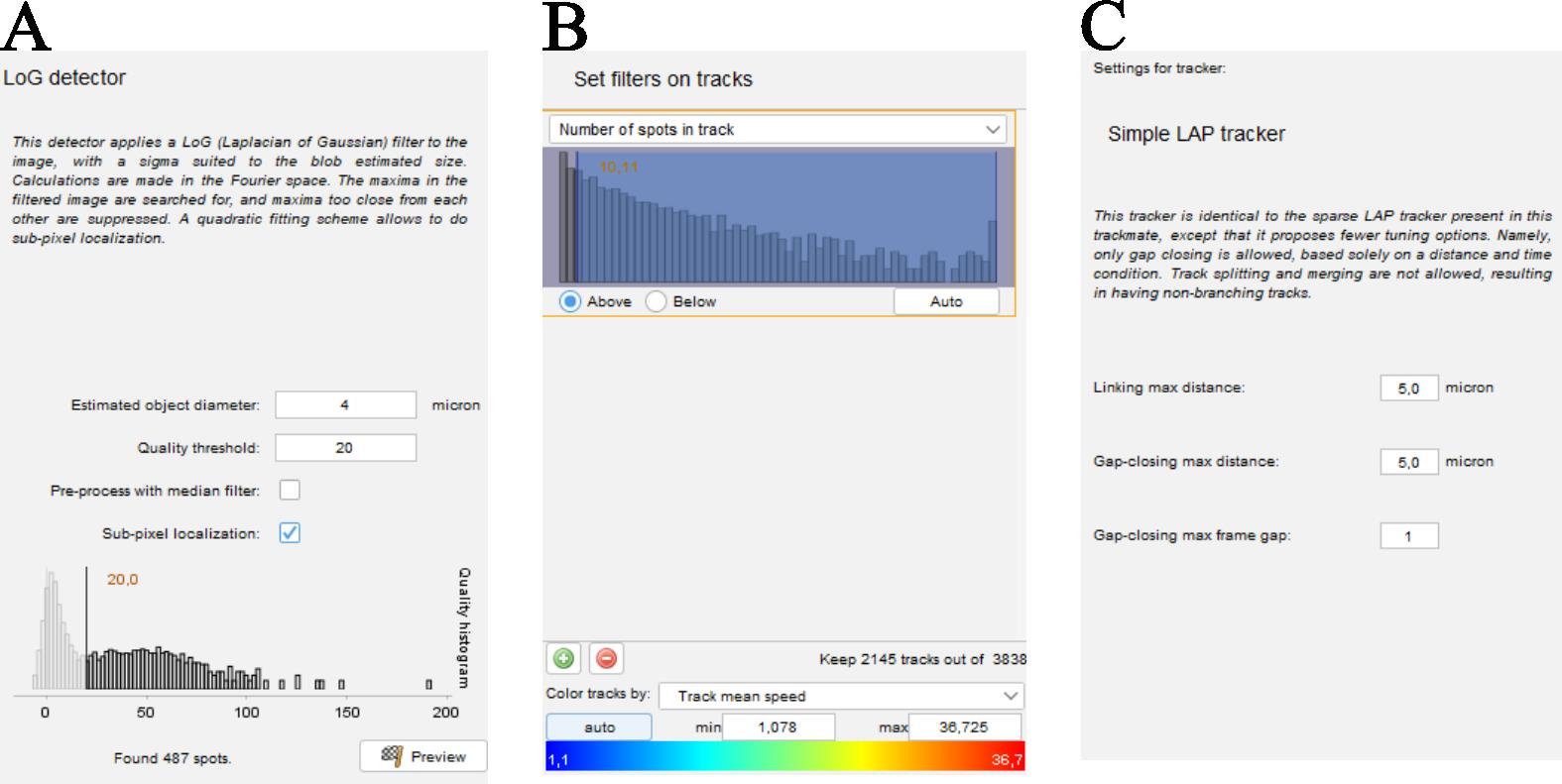
Figure 2. Screenshots taken during film analysis to determine bacterial trajectories using the TrackMate plugin. (A) Window in which you can enter the size and quality factor for detecting bacteria on each of the images. (B) Window that opens when you need to enter the parameters that will be used to link the particles detected between two successive images and thus reconstruct its trajectory. (C) Window at which filters can be applied to the trajectories. We have chosen to keep only trajectories containing more than 10 positions.
B. Suppression of the non-motile bacteria from the tracks, determination of the accumulation length and diffusion coefficient from the trajectories, and determination of the chemotactic velocity
1. Treat the CSV files with a tabulator. We recommend using the Pandas library in Python. It is also possible to use Microsoft Excel. A simplified version of the Python code we used is available in File S1.
2. The CSV file lists the trajectories by index
3. Non-motile bacteria are in the liquid, while others stick to the surface and are recorded during the image acquisition. As this sub-population shows no chemotaxis, it is necessary to remove these bacteria from the list of trajectories obtained previously before conducting a statistical analysis of the trajectories. This is done by removing the trajectories
4. Determination of the diffusion coefficient from the average value of
a. The persistence time measures the time over which the orientation of a bacterium's trajectory remains identical [9]. Over longer times, the trajectory is equivalent to that of a random walker. This time is obtained from the velocity correlation function calculated as [3]:
(4)
For particles randomly exploring their environment, the correlation function decays like (5), where τ is the correlation time we look for and vy is the average velocity of all the particles along the y axis estimated in step B2 (Data analysis).
b. When the correlation function is divided by
c. The diffusion coefficient is [9].
5. Determination of the accumulation characteristic length λ from the positions of the bacteria in the channel.
a. Segment the image along the y-axis into 20 μm wide bins and measure the bacterial density by counting the number of spots inside each bin to finally get the density distribution.
b. The concentration of bacteria in the stationary regime decays exponentially and is described by the function , where y0 is the upper boundary location, b0 is the bacterial density at y0, and λ is the characteristic accumulation length. Measure y0 and b0 from the image and calculate λ through the regression of the distribution by the function.
6. The chemotactic velocity vc is obtained from Eq. (2) using the diffusion coefficient obtained in step B4 (Data analysis) and the accumulation length obtained in step B5 (Data analysis). The chemotactic velocity is measured for an average concentration and a gradient , where L = 1 mm is the distance between the channels containing the chemoattractant.
7. The chemotactic susceptibility χ(c) is obtained from Eq. (3) by dividing vc by ∇c. The variation of χ(c) with c can be obtained by performing experiments with various couples (c,∇c).
Validation of protocol
We applied this protocol by placing a suspension of E. coli in the central channel between two channels containing 200 and 0 μM of α-methyl-aspartate in the motility buffer. We waited 30 min for the gradient to be established before starting to acquire the films. For this experiment, we then have c = 100 μM and ∇c = 200 μM/mm. Figure 3 shows the first image of three films recorded during the experiment. In the first image, the bacteria, which appear as white dots, are evenly distributed across the image.
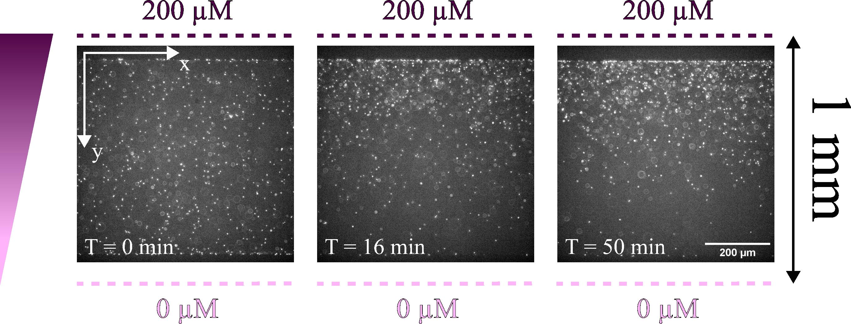
Figure 3. Images acquired at three different times (0, 16, and 50 min). The images show the central channels where the bacteria suspension was injected. The observation is done with a 20× objective. The bacteria appear as white dots. Over time, we can see that the bacteria have moved upward and are accumulating on the side closest to the channel containing the chemoattractant.
After a few minutes, the bacteria are more numerous at the top of the image, on the side where the chemoattractant is present. This is shown quantitatively in Figure 4A, where we plotted the profiles b(y) obtained after the image treatment. The adjustment of each profile by an exponential function gives a decay length that we plot as a function of the time at which the films were recorded (Figure 4C). The decay length changes very little over time, indicating that the bacterial concentration profile reaches a stationary regime within a few minutes and no longer evolves over time. The average decay length measured is λ = 130 ± 10 μm (Figure 4C).
Next, each film was processed to determine the velocity correlation function Cy(Δt) (see Figure 4B). Fitting it gives the correlation time τ, which, combined with the average velocity of the bacteria along the y-axis vy, gives the diffusion coefficient . The diffusion coefficient as a function of time is shown in Figure 4D. The diffusion coefficient shows little variation over time; we obtained D = 260 ± 30 μm2/s. The accumulation length λ and diffusion coefficient D are then used to determine the chemotactic velocity vc for each film. This is shown as a function of time in Figure 4E. The chemotactic velocity also shows little variation with time; we found: vc =1.9 ± 0.4 μm/s.
The experiment was continued with different concentrations c1 and c2 in the channels, which makes it possible to explore other pairs of parameters (c,∇c) and their influence on the chemotactic velocity. Figure 5 shows, in a log-log representation, the chemotactic susceptibility as a function of c. Each point corresponds to one experiment. Outside the window of c represented in Figure 5, no chemotactic responses were detected. The central part of the data are adjusted by a line indicating that over this region we have with χ0 = 490 ± 40 μm2/s/μM.
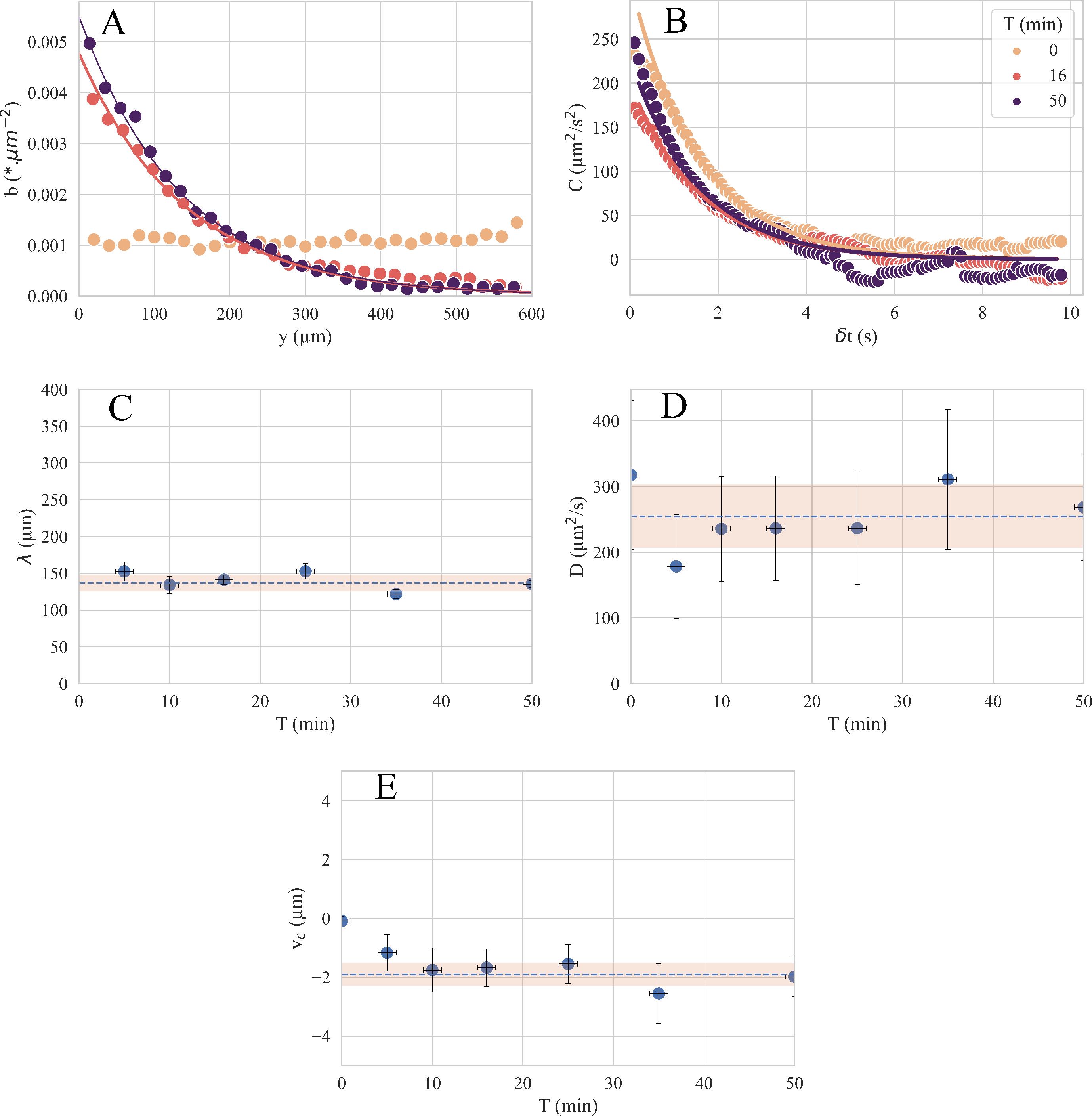
Figure 4. Data processing to obtain a chemotactic velocity. (A) Bacterial concentration profiles b(y) and (B) velocity correlation function Cy(Δt) measured at three different times during one experiment. The solid lines are exponential fit that determine a) the decay length λ and b) the persistence time τ. (C) Time evolution of the decay length λ. (D) Time evolution of the diffusion . (E) Chemotactic velocity vc obtained by Eq. (2) that combines the decay length λ and the diffusion coefficient D. The data are from an experiment with c = 100 μM and ∇c = 200 μM/mm.
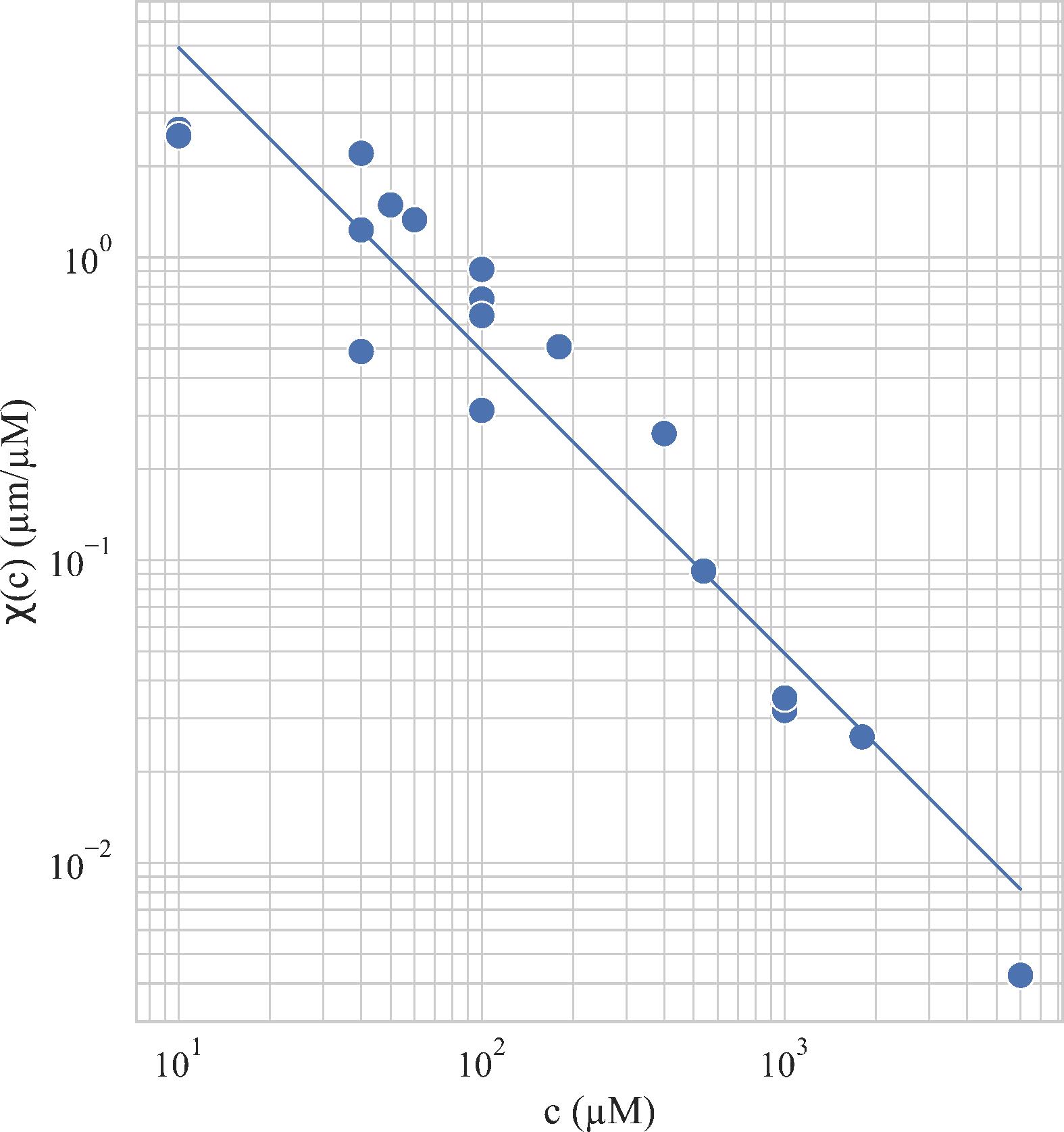
Figure 5. Evolution of the chemotactic coefficient χ(c) as a function of the average concentration c. For concentrations below 1 and above 104 μM, no chemotactic response was detected. Solid line: with χ0 = 490 ± 40 μm2/s/μM.
General notes and troubleshooting
General notes
1. Any remaining bubbles in the channels might cause residual flow that will bias the experiment. Special care is needed to avoid them during the different steps.
2. The settings are for fluorescent strains of bacteria. If the bacteria are not fluorescent, an alternative is to use phase contrast image acquisition. In this case, tracking might require a treatment to eliminate artifacts in the images.
3. The bacteria density profile does not evolve anymore after 5–20 min, depending on the experiment. We recommend waiting for 20 min before starting the image acquisition.
4. The acquisition frequency has to be adjusted so that the typical displacement of a bacteria between two successive images is of the order of 2 pixels. For a characteristic swimming velocity of bacteria of ~10 μm/s, an acquisition frequency of 0.1 s fits this requirement.
5. Films can be acquired at different heights above the agar. We did not observe any effect of this parameter on the estimation of χ(c).
6. If you would like to reuse the PDMS mold, then:
a. Before dismounting the microfluidic cell, flush water into the device.
b. After dismounting, clean the PDMS with ethanol, dry it, and remove the dust on the surface with tape.
c. Finally, stick some tape on the PDMS mold. The mold can then be kept and eventually reused.
7. Swimming velocity or diffusion coefficient measurements are also a good way of identifying batch-to-batch variation in bacterial suspension.
Troubleshooting
Problem 1: The liquid PDMS foams out of the container.
Cause: Bubbles develop in the vacuum chamber and form a foam.
Solution: Break the vacuum regularly.
Problem 2: The agar layer breaks when manipulated.
Cause: The layer is still too warm.
Solution: Make sure the plate is cold enough. It should have some condensation on it.
Problem 3: Flow in the central channel.
Cause 1: Agar delamination on the extrema after 3 h under the microscope.
Solution 1: Wet the agar every hour by pouring pure water drops around the chip.
Cause 2: Motion and vibration of the tubings due to air conditioning.
Solution 2: Put a valve between the microtube containing bacteria and the chip.
Cause 3: Deformation of the PDMS mold due to the tubing.
Solution 3: Do not insert the tubing too deep into the PDMS molding. The molding should be ~1 cm thick so that it can hold the tubing and still remain flat.
Supplementary information
The following supporting information can be downloaded here:
1. File S1. Python Analysis script
Acknowledgments
This work was funded by the CNRS MITI (Mission pour les Initiatives Transverses et Interdisciplinaires) 80|PRIME – 2021 program. We also acknowledge Ahmed et al. [1,5] for the work they conducted, which inspired the current paper.
Competing interests
The authors have no conflict of interest to report.
References
- Ahmed, T., Shimizu, T. S. and Stocker, R. (2010). Bacterial Chemotaxis in Linear and Nonlinear Steady Microfluidic Gradients. Nano Lett. 10(9): 3379–3385.
- Keller, E. F. and Segel, L. A. (1971). Model for chemotaxis. J Theor Biol. 30(2): 225–234.
- Bouvard, J., Douarche, C., Mergaert, P., Auradou, H. and Moisy, F. (2022). Direct measurement of the aerotactic response in a bacterial suspension. Phy Rev E. 106(3): e034404.
- Pfeffer, W. (1888). Untersuchungen aus dem botanischen Institut zu Tübingen. (Vol. 2). In: Engelmann, W. 1881–1888
- Ahmed, T., Shimizu, T. S. and Stocker, R. (2010). Microfluidics for bacterial chemotaxis. Integr Biol. 2: 604–629.
- Stehnach, M., Henshaw, R., Floge, S. and Guasto, J. (2024). Multiplexed Microfluidic Platform for Parallel Bacterial Chemotaxis Assays. Bio Protoc. 14(1352): e5062.
- Parkinson, J. S. (1978). Complementation analysis and deletion mapping of Escherichia coli mutants defective in chemotaxis. J Bacteriol. 135(1): 45–53.
- Tinevez, J. Y., Perry, N., Schindelin, J., Hoopes, G. M., Reynolds, G. D., Laplantine, E., Bednarek, S. Y., Shorte, S. L. and Eliceiri, K. W. (2017). TrackMate: An open and extensible platform for single-particle tracking. Methods. 115: 80–90.
- Lovely, P. S. and Dahlquist, F. (1975). Statistical measures of bacterial motility and chemotaxis. J Theor Biol. 50(2): 477–496.
Article Information
Publication history
Received: Sep 11, 2024
Accepted: Dec 8, 2024
Available online: Dec 31, 2024
Published: Feb 20, 2025
Copyright
© 2025 The Author(s); This is an open access article under the CC BY-NC license (https://creativecommons.org/licenses/by-nc/4.0/).
How to cite
Gargasson, A., Douarche, C., Mergaert, P. and Auradou, H. (2025). Quantifying Bacterial Chemotaxis in Controlled and Stationary Chemical Gradients With a Microfluidic Device. Bio-protocol 15(4): e5184. DOI: 10.21769/BioProtoc.5184.
Category
Bioinformatics and Computational Biology
Biological Sciences > Microbiology > Microbial communities
Microbiology > Microbial physiology > Chemotaxis
Do you have any questions about this protocol?
Post your question to gather feedback from the community. We will also invite the authors of this article to respond.