Microdissection and Single-Cell Suspension of Neocortical Layers From Ferret Brain for Single-Cell Assays

Materials and reagents

Biological materials

1. Pregnant sable ferret (Mustela putorius furo) (Euroferrets, Denmark)

1. Blue ultrasound gel (Transonic, catalog number: TOG04)

2. Sodium chloride (NaCl) (Sigma-Aldrich, catalog number: S9888)

3. Sodium phosphate dibasic (Na₂HPO₄) (Sigma-Aldrich, catalog number: S3264)

4. Potassium chloride (KCl) (VWR, catalog number: 26759.291)

5. Potassium dihydrogen phosphate (KH₂PO₄) (VWR, catalog number: 26925.295)

6. MACS neural tissue dissociation kit (P) (Miltenyi Biotec, catalog number: 130-092-628)

7. Leibovitz’s 1× L-15 medium with L-glutamine, without phenol red (Gibco, catalog number: 21083027)

8. SeaPlaque agarose (Lonza, catalog number: 50100)

9. Bovine serum albumin (BSA) (Sigma-Aldrich, catalog number: A7906)

10. 1× Phosphate buffered saline (PBS) without CaCl₂/MgCl₂ pH 7.4 (Gibco, catalog number: 10010023)

11. RNaseZap RNase decontamination solution (Invitrogen, catalog number: AM9780)

12. Anesthetic/analgesic cocktail: xylazine (Karizoo, trade name: Xylasol 20 mg/mL, catalog number: 579700.7), ketamine (VetViva Richter, trade name: Ketamidor 100 mg/mL, catalog number: 580393.7), buprenorphine (VetViva Richter, trade name: Bupaq 0.3 mg/mL, catalog number: 578816.6)

13. Saline solution (NaCl 0.9%) (Interapothek, catalog number: 208978)

14. 1× Hank’s balanced salt solution (HBSS) without CaCl₂/MgCl₂/phenol red (Gibco, catalog number: 14175095)

15. Ethanol absolute (VWR, catalog number: 20821.365P)

16. 0.4% Trypan blue stain (Invitrogen, catalog number: T10282)

1. 10× Phosphate buffered saline (PBS) stock solution (see Recipes)

2. 1× PBS (see Recipes)

3. Cell collection medium (see Recipes)

1. 10× PBS stock solution (1 L)

   Reagent	Final concentration	Quantity or Volume
   NaCl	1.37 M	80 g
   Na2HPO4	100 mM	14.4 g
   KCl	27 mM	2 g
   KH2PO4	18 mM	2.4 g
   Distilled H2O	n/a	1 L*
   Total	n/a	1 L

   *Dilute reagents in 800 mL, bring solution pH to 7.4, and top off to 1 L.




2. 1× PBS (1 L)

   Reagent	Final concentration	Quantity or Volume
   PBS 10×	1×	100 mL
   Distilled H2O	n/a	900 mL
   Total	n/a	1 L




3. Cell collection medium (50 mL)

   Reagent	Final concentration	Quantity or Volume
   BSA	0.04% (w/v)	0.02 g
   PBS (without CaCl2/MgCl2, pH 7.4)	1×	50 mL
   Total	n/a	50 mL

   The medium should be freshly prepared and filtered on the day of the experiment.

Laboratory supplies

1. Glass Pasteur pipettes (Fisher Scientific, catalog number: FB50253)

2. 0.5 mL PCR tubes (Eppendorf, catalog number: 0030124537)

3. 2 mL DNA LoBind tubes (Eppendorf, catalog number: 0030108078)

4. 15 mL centrifuge tubes (Corning, catalog number: 430791)

5. 50 mL centrifuge tubes (Corning, catalog number: 430829)

6. 40 μm PluriStrainer mini cell strainers (PluriSelect, catalog number: 43-10040-40)

7. 0.22 μm syringe filter (VWR, catalog number: 514-1263)

8. 50 mL sterile syringe (BD, catalog number: 300865)

9. Pipetman P1000 tips (Daslab, catalog number: 162222)

10. Pipetman P200 tips (Daslab, catalog number: 162001)

11. Pipetman P20 tips (Daslab, catalog number: 162001)

12. Permanent marker pen (Sarstedt, catalog number: 95.954)

13. 100 mm × 15 mm sterilized Petri dishes (JetBiofil, catalog number: TCD010100)

14. Ice buckets

15. 500 mL PYREX griffin low-form beaker (Corning, catalog number: 1000J-500)

16. 1 mL sterile syringe (ENFA, catalog number: JS1)

17. 10 mL sterile syringe (BD, catalog number: 307736)

18. Microlance 3 hypodermic needles 25 G × 5/8'', 16 × 0.5 mm (BD, catalog number: 300600)

19. Microlance 3 hypodermic needles 30 G × 1/2'', 13 × 0.3 mm (BD, catalog number: 304000)

20. Polypropylene laboratory tray (Vitlab, catalog number: 72298)

21. Single-edge razor blade (KBC, catalog number: 1-909-11036)

22. Double-edge razor blade (Gillette Platinum, catalog number: 21377003)

23. Peel-A-Way embedding molds truncated - T12 (Polysciences, catalog number: 18986-1)

24. Peel-A-Way embedding molds rectangular - R30 (Polysciences, catalog number: 18646B-1)

25. Super Glue-3 (Loctite, catalog number: 2640076)

26. LDPE Pasteur pipette (Fisher Scientific, catalog number: 747760)

27. 20 μL ZEROTIP pipette micro tip with filter (JetBiofil, catalog number: PMT252020)

28. 2 mL floating tube rack (Sigma-Aldrich, catalog number: R7776-5EA)

29. Digital timer (Scharlau, catalog number: 038-000566)

30. Pipetman P10 tips (Daslab, catalog number: 163030)

31. 0.2 mL PCR tubes (Eppendorf, catalog number: 0030124332)

32. Hand tally counter (VWR, catalog number: 710-0935)

33. Countess cell counting chamber slides (Invitrogen, catalog number: C10228)

Equipment

1. Ultrasound system (SonoSite, model: MicroMaxx)

2. Distilled water (H₂O) (Milli-Q, model: IQ-7000)

3. pH meter (Crison, model: Basic 20+)

4. Autoclave (Tuttnauer, model: 2540M)

5. Bunsen burner (Carl Roth, catalog number: CK29.1)

6. Drying oven (POL-EKO, model: SLW400)

7. Straight, sharp tips, fine dissecting scissors (Fine Science Tools, catalog number: 14060-09)

8. Straight, super fine tips dissecting forceps (Fine Science Tools, catalog number: Dumont #5SF 11252-00)

9. Micro spoon spatulas (RSG Solingen, catalog number: 80.025.150)

10. Micro flat-ended spatula (RSG Solingen, catalog number: 80.038.150)

11. 15° straight, sharp pointed tips, microsurgical stab knives (MSP, catalog number: 72-1501)

12. Straight, sharp/blunt tips dissecting scissors (Fine Science Tools, catalog number: 14001-18)

13. Pipetman P1000 (Gilson, catalog number: F144059M)

14. Pipetman P200 (Gilson, catalog number: F144058M)

15. Pipetman P20 (Gilson, catalog number: F144056M)

16. Laminar flow hood (Telstar, model: CytoStar)

17. Water bath at 42 °C (MRC, catalog number: WBO-100)

18. Dissecting scope with incident illumination (Leica, model: M60)

19. Vibratome (Leica, model: VT1000 S)

20. Dissecting scope with transmitted illumination (Leica, model: MS5)

21. Vortex mixer (Labnet)

22. Water bath at 37 °C (MRC, catalog number: WBO-200)

23. Microcentrifuge (Labnet, model: Spectrafuge 24D)

24. Blaubrand Neubauer counting chamber (Brand, catalog number: 718605)

25. Pipetman P10 (Gilson, catalog number: F144055M)

26. Inverted microscope (Leica, model: DM IL)

27. Countess II FL automated cell counter (Invitrogen, catalog number: AMQAF1000)

Procedure

1. Material preparation before the day of the experiment

   1. Perform an abdominal ultrasound on the jill 27–30 days after mating to verify a successful pregnancy and the number of kits. Plan the number of samples to be isolated during the experiment (see General note 1).

   2. Prepare 1 L of 10× PBS stock solution, autoclave it, and store at room temperature (RT).

   3. Fire-polish glass Pasteur pipettes to round off sharp edges without significantly decreasing the size of the opening. Prepare one glass Pasteur pipette per dissected sample. Autoclave.

      Critical: Dry autoclaved fire-polished pipettes for 2 days in the oven to remove any remaining moisture inside them, as microdissected tissue pieces may stick to wet pipettes.

   4. Autoclave dissecting material: two fine dissecting scissors, three super fine dissecting forceps, two micro spoon spatulas, one micro flat-ended spatula, and 1 L of 1× PBS solution.

   5. Reconstitute, aliquot, and store MACS kit reagents to be ready to use according to manufacturer’s instructions.




2. Material preparation on the day of the experiment

   1. Sterilize microsurgical stab knives, sharp/blunt tip dissecting scissors, 0.5 and 2 mL tubes, 15 and 50 mL centrifuge tubes, 40 μm strainers, 0.22 μm syringe filter, 50 mL syringe, P1000, P200, and P20 pipettes and tips, and a marker. Do this by exposure to UV light inside a laminar flow hood for 30 min.

   2. Aliquot 500 mL of cold (4 °C) L-15 medium in 50 mL centrifuge tubes inside the flow hood and store at 4 °C.

   3. Prepare 50 mL of fresh 4% low melting-temperature agarose in autoclaved 1× PBS. Keep melted agarose in a water bath at 42 °C.

   4. Prepare 50 mL of fresh cell collection medium and filter inside the flow hood using a sterile 0.22 μm syringe filter attached to a sterile 50 mL syringe.

   5. Clean lab benches with RNase decontamination solution. Four benches will be required: one to obtain embryonic day 34 (E34) ferret embryos by cesarian section or to keep postnatal day 1 (P1) ferret kits, one to extract the brains, and two neighboring benches, one to slice the brains and the other to microdissect the brain slices.

   6. Place equipment on clean benches: dissecting scope equipped with incident light source and two empty 100 mm Petri dishes for brain extraction, vibratome with crushed ice inside its cooling bath, and dissecting scope equipped with transmitted illumination for slice microdissection.

   7. Prepare five ice buckets: one big and deep that contains a 500 mL beaker with 350 mL of autoclaved 1× PBS, one big and flat that can hold up to six Petri dishes of 100 mm diameter, one small and flat with space for two Petri dishes of 100 mm diameter, one small for 2 mL tubes, and one big and deep to replace melted ice in the vibratome’s cooling bath.




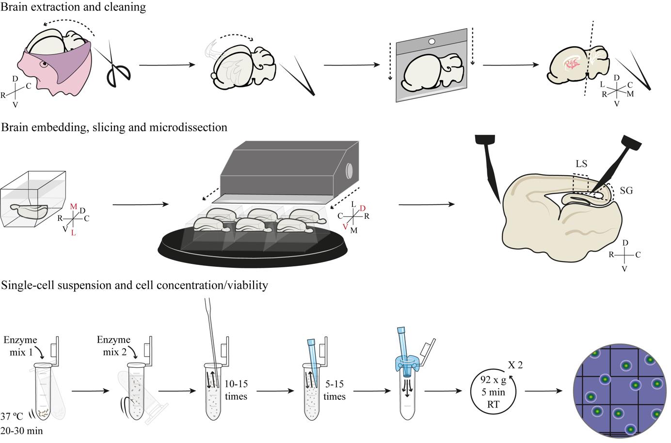
3. Brain extraction and cleaning

   Time frame to complete this section: ~1 h 20 min

   1. Inject the cocktail of anesthetic/analgesic to overdose the timed-pregnant jill (if obtaining samples from E34 embryos), or the P1 kit (if obtaining samples from early postnatal ferrets).

      1. Administer xylazine (0.05–0.1 mL/kg), ketamine (0.05–0.15 mL/kg), and buprenorphine (0.03–0.06 mL/kg) in a single injection via intramuscular (IM) administration. Wait until there is no sensory response.

         Note: For pregnant jills, wait a minimum of 6 min to ensure a complete anesthetic/analgesic effect.

      2. Administer 16.67% (v/v) sodium pentobarbital diluted in saline solution via intraperitoneal (IP) administration. Wait 10 min for full effect.

      Note: Both steps C1a and C1b are carried out for pregnant jills and P1 kits, with identical doses per animal’s body weight.

   2. Place the deeply anesthetized pregnant jill on a tray.

   3. Perform a cesarean section using sterilized sharp/blunt-tip dissecting scissors, extract the uterine horns, and place them inside the 500 mL beaker with ice-cold PBS. Cut the diaphragm and the heart right atrium of the jill for final euthanasia.

   4. Extract the embryos by cutting open the uterine horns longitudinally and piercing the amniotic sac using the autoclaved fine dissecting scissors. Keep the embryos in ice-cold PBS.

   5. Fill the 100 mm Petri dishes for brain extraction with ice-cold L-15 aliquoted medium.

   6. Decapitate the E34 embryo or P1 kit by cutting along the base of the skull with the fine or the sharp/blunt-tip dissecting scissors, respectively.

   7. Place the head in the 100 mm Petri dish filled with ice-cold L-15 medium under the dissecting scope with incident light.

   8. Hold the head still for brain extraction with the autoclaved super fine dissecting forceps, by piercing the eyes rostro-caudally (Figure 1A).

      
      

      
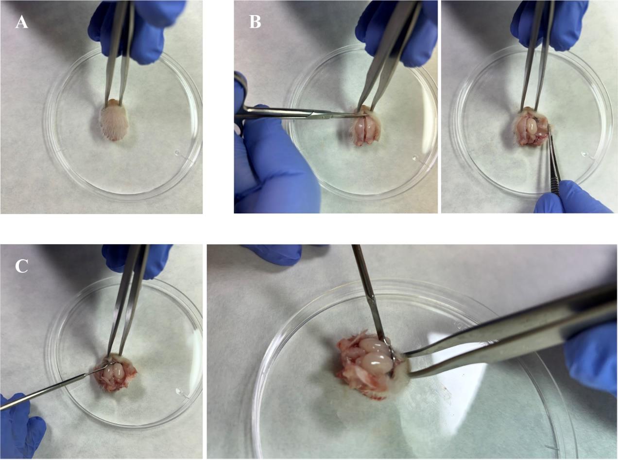
      Figure 1. Craniotomy for brain extraction. A. Immobilize the head by carefully piercing the eyes with the super fine dissecting forceps. B. Cut the snout open by making incisions on both sides of the head. C. Shell out the olfactory bulbs by carefully inserting a micro-spoon spatula into the rostral side of the opened skull.

      
      

   9. Using a new pair of autoclaved fine dissecting scissors, cut along the dorsal midline through the skin and membranous skull, from the back of the head to the snout. For this operation, place the sharp tips of the dissecting scissors upward and the blade slightly parallel to the surface of the skull, to avoid piercing or cutting the brain’s surface.

      Note: To keep the surface of the brain intact, the skin layer can be cut first and peeled away to the sides; then, cut both pieces out and proceed with the membranous skull.

   10. At the level of the snout, extend the midline cut to both sides of the head, to open the skull and access the brain (Figure 1B).

   11. Insert a micro spoon spatula rostrally to detach the olfactory bulbs (OBs) from the skull (Figure 1C).

   12. Turn the head over to extract the brain from the skull. Use the micro spoon spatula to carefully release it from any remaining tissue attachments and the fine dissecting scissors to cut the cranial nerves on the ventral side.

   13. Transfer the extracted brain to the other 100 mm Petri dish filled with ice-cold L-15 using the micro spoon spatula.

   14. Remove the meninges (these appear as a transparent film) using two new autoclaved super fine dissecting forceps. Pierce them at the level of the OBs and carefully pull them out rostrocaudally, taking care to avoid touching the brain’s surface. This should be done on both brain sides (dorsal and ventral) sequentially.

       Critical: Avoid pulling the meninges with excessive force, or else tissue will deform and damage, particularly at the caudal cortex. Incomplete removal of the meninges may also cause deformation of the tissue during vibratome cutting.

       Note: Stabilize the floating brain by pinching the remnants of the spinal cord and cerebellum.

   15. Split the brain along the midline into its hemispheres using a single-edged razor blade. Make a clean cut in one fell swoop. Then, move the blade back and forth without lifting it until the hemispheres separate completely.

   16. Remove the choroid plexus from the lateral ventricle and any meninges debris from the caudal cortex using the super fine dissecting forceps.

       Critical: Avoid pulling the choroid plexus with excessive force to prevent tissue deformation. Incomplete removal of the choroid plexus may also cause deformation of the tissue during vibratome cutting.

   17. Clamp the remnants of the spinal cord and cerebellum with one of the dissecting forceps. Close the tips from the second forceps and move them down along the edge of the clamping forceps to cut out the remaining.

   18. Depending on the single-cell assay to carry out, and hence the required cell concentration (see General note 1), repeat steps C5–17 to obtain other E34 ferret embryos or steps C1 and C5–17 for other P1 kits.




4. Brain embedding and slicing

   Time frame to complete this section: ~1 h 50 min

   1. Label a histology embedding mold (whose size is in accordance with the brain size) with the animal number and L (left) or R (right) according to the brain hemisphere.

   2. Fill the mold with freshly prepared 4% low-melting temperature agarose.

   3. Transfer one brain hemisphere into the mold using the micro-spoon spatula, with the minimum accompanying liquid.

   4. Rotate the brain hemisphere inside the liquid agarose with a P200 pipette tip by describing circles around the tissue in all directions, but without touching it.

      Critical: Multiple turns of the tissue in all directions within the agarose are essential to build a complete coating around it and to avoid its popping out during vibratome cutting later on.

   5. Before the agarose solidifies, place the brain hemisphere horizontally at the bottom of the mold with its lateral side facing down and its medial side facing up.

   6. Place the mold on ice until it solidifies completely.

   7. Extract the solidified agarose block containing the brain hemisphere from the mold and place it on the lid of a 100 mm Petri dish. The medial side of the hemisphere should face the base of the pyramid. Using the single-edged razor blade, cut the sides of the agarose block into the shape of a truncated square pyramid.

   8. Repeat steps D1–7 for the other hemispheres.

      Note: Up to six hemispheres from E34 ferret embryos or up to four hemispheres from P1 kits can be vibratome-cut in one go.

   9. Glue the truncated pyramids on the vibratome’s specimen disk. To harden the glue quickly and improve the truncated pyramid attachment, add drops of ice-cold L-15 to the base of the pyramids with an LDPE Pasteur pipette. Given that the medial side of the hemisphere is facing the pyramid’s base, the lateral side of the cerebral cortex should face upward and will be the first to be cut.

      Critical: The corpus callossum on the ventral side of the brain has a harder consistency than the cortical cell bodies. Therefore, the softer tissue should be cut before to avoid being pushed by the callossum.

   10. Tighten the specimen disk to the buffer tray, fill it with ice-cold L-15 medium, place the knife holder with an unused blade from the double-edged razor blades, set the sectioning parameters on the vibratome, and place new ice inside the cooling bath.

   11. Label 100 mm Petri dishes (as many as brain hemispheres to be cut), fill them with ice-cold L-15 medium, and place them on the big flat ice bucket.

   12. Cut the brain hemispheres from E34 embryos or P1 kits.

       1. Make 300 μm thick slices at a vibratome speed of 2, frequency 5 to 6.

       2. Use two micro spatulas (one spoon and one flat-ended) to collect each slice and place them in their corresponding Petri dishes.

       3. Check the slices under the dissecting scope equipped with transmitted light until the regions of interest (ROIs) [the prospective splenial gyrus (SG) and lateral sulcus (LS), in our case] come into sight.




5. Microdissection

   Time frame to complete this section: ~2 h 15 min for E34 embryos or ~1 h 40 min for P1 kit.

   1. Set a 100 mm Petri dish with the identified ROIs in the small flat ice bucket.

   2. Replace the Petri dish set aside with a new dish, so brain slices from that hemisphere can still be collected during the microdissection.

   3. Place the Petri dish with the identified ROIs under the dissecting scope with transmitted illumination. Using two microsurgical stab knives, carefully drag the slice of interest by its surrounding agarose and place it at the center of the field of view.

   4. Microdissect the first ROI: prospective SG (Figure 2A).

      1. Hold the slice by the surrounding agarose with one knife and use the other knife to make a horizontal cut at the most caudal end of the cortex, right next to the hippocampal formation.

      2. Without lifting the knife that holds the agarose, use the second knife to make a second cut at a 45° angle with respect to the previous cut.

         Critical: These two cuts will detach the prospective SG from the agarose. This piece of tissue is very small, so do not miss sight of it.

         Critical: A lack of precision when making the horizontal cut next to the hippocampal formation, or at a 45º angle, may lead to the isolation of unwanted cells from neighboring cortical areas, which may be difficult to discard during subsequent analyses.

      
      

      
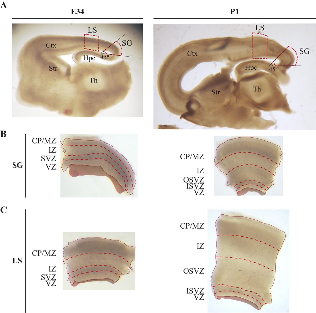
      Figure 2. Neocortical areas and layers to microdissect. A. Example of live parasagittal slices from the brains of embryonic day (E) 34 and postnatal day (P) 1 ferrets with lateral sulcus (LS) and splenial gyrus (SG) outlined. Ctx, cortex; Str, striatum; Hpc, hippocampus; Th, thalamus. B, C. Tissue microdissections of the SG (B) and LS (C) from the two developmental stages with neocortical layers depicted. CP/MZ, cortical plate/marginal zone; IZ, intermediate zone; SVZ, subventricular zone; OSVZ, outer subventricular zone; ISVZ, inner subventricular zone; VZ, ventricular zone. Figure modified from [8].

   
   

   5. Set aside the slice missing the prospective SG and focus on the dissected SG at the highest magnification of the dissecting scope.

   6. Microdissect the most apical cortical layer from the first ROI, the ventricular zone (VZ) (Figure 2B).

      1. Use one knife to hold the dissected slice piece by an unwanted part of the tissue, in our case the top half.

      2. Carefully make a clean cut in one fell swoop of the layer that is most cell-dense and opaque, extending from the side of the cortex limiting with the ventricular cavity (see General note 4). This covers approximately 3/10 of the cortex total thickness in E34 embryos and 1/10 in P1 kits.

         Critical: The VZ is slightly concave, so make your cut such that it contains the whole thickness of the VZ. Excess tissue can be trimmed off afterward.

         Critical: Cut with moderate force to avoid pushing away the dissected thin layer and possibly losing it in the medium.

      1. Turn the VZ around, prick the layer, and trim away any unwanted tissue.

      2. Cut the dissected VZ into small pieces.

         Note: Increasing the surface area of the dissected tissue will enable a larger contact between the tissue and the dissociating enzyme later on.

         Critical: Do not mix the VZ pieces with the previously trimmed chunks.

   7. Use a P20 pipette with low retention, RNase-free filter-tip to aspirate the VZ pieces with as little medium as possible. Transfer the pieces to a 2 mL tube, label it, and put it in the small ice bucket.

      Critical: Check the pipette tip under the dissecting scope to make sure that the pieces have not stuck to its walls or opening. If that is the case, see the Troubleshooting section, problem 1.

   8. Microdissect the second cortical layer from the first ROI, the outer subventricular zone (OSVZ) (Figure 2B).

      Note: The OSVZ emerges at E34, therefore this layer is not yet present in E34 ferret embryos but is developed in P1 kits (Figure 3).

      1. Again, use one knife to hold the dissected slice piece by the top half of the tissue.

      2. Trim away the remnants of the cell-dense layer at the apical side.

         Note: This layer is the inner subventricular zone (ISVZ). At P1, it has the thickness of the VZ; however, part of it has probably been dissected with the VZ and was later trimmed off.

      3. Carefully make a clean cut in one fell swoop of the bottom half still left of the cortex's total thickness. It is a translucent layer, although denser than the layer directly on top [the intermediate zone (IZ)], especially its upper third. The lower 2/3 of this layer displays cells radially organized in ribbons (see General note 4).

      4. Cut the dissected OSVZ into small pieces.

         Note: Increasing the surface area of the dissected tissue will enable a larger contact between the tissue and the dissociating enzyme later on.

         Critical: Do not mix the OSVZ pieces with the previously trimmed ISVZ.

      
      

      
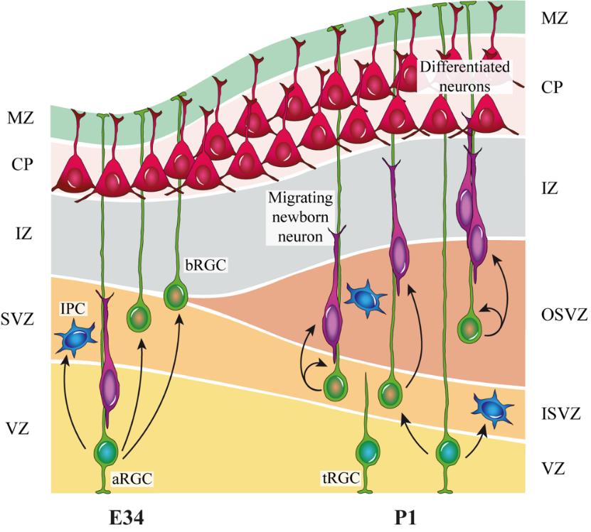
      Figure 3. Layer and cellular composition along cortical development. Layer composition at embryonic day (E) 34, when apical radial glia cells (aRGC) in the ventricular zone (VZ) self-consume to generate basal progenitors. At this stage, the first basal radial glia cells (bRGC) that initiate the outer subventricular zone (OSVZ) are produced. At postnatal day (P) 1, the bRGC from the OSVZ self-amplifies and, contrary to the inner subventricular zone (ISVZ), arises independently from aRGC. IPC, intermediate progenitor cell; tRGC, truncated radial glia cell; MZ, marginal zone; CP, cortical plate; IZ, intermediate zone; SVZ, subventricular zone. Figure modified from [16].

   
   

   9. Use the P20 pipette with low retention, RNase-free filter-tip to aspirate the OSVZ pieces with as little medium as possible. Transfer the pieces to a 2 mL tube, label it, and put it in the small ice bucket.

      Critical: Check the pipette tip under the dissecting scope to be sure that the pieces have not stuck to its walls or opening. If that is the case, see the Troubleshooting section, problem 1.

   10. Select the lowest magnification in the dissecting scope, focus the slice from which the prospective SG was microdissected, and trim away the following piece of cerebral cortex with a similar size as the microdissected SG.

   11. Microdissect the second ROI, prospective LS (Figure 2A).

       Hold the slice by the surrounding agarose with one knife and use the other one to make a vertical cut over the cortex overlying the hippocampal region immediately caudal to the dentate gyrus.

       Critical: This cut will detach the prospective LS from the agarose, so do not mistake it with the previous discarded piece of tissue.

   12. Focus on the dissected LS at the highest magnification of the dissecting scope.

   13. Repeat steps E6–7 to isolate the most apical cortical layer from the second ROI, VZ from LS (Figure 2C).

   14. Repeat steps E8–9 to isolate the second cortical layer from the second ROI, OSVZ from LS (Figure 2C).

   15. Microdissect the layers from all the vibratome slices containing the ROIs: 2–3 slices per hemisphere from E34 embryos or 4–5 slices per hemisphere from P1 kits.

       Note: Pool the VZ pieces from 2–3 E34 embryos in the same 2 mL tube to obtain the optimal cell concentration range; see General note 1.




6. Single-cell suspension

   Time frame to complete this section: ~1 h 20 min

   1. For each sample to be processed, prepare 1,950 μL of enzyme mix 1 from the MACS kit inside the laminar flow hood by adding the following components:

      Buffer X, 1,900 μL

      Enzyme P, 50 μL

      Vortex and prewarm the mixture in a water bath at 37 °C for 20 min before use.

   2. For each sample to be processed, pre-wet a 40 μm strainer sitting in a 2 mL tube with 1× HBSS.

      Note: Wetting the strainer membrane helps to reduce cell adhesion.

   3. Carry the samples on ice to the flow hood.

   4. Add 1,950 μL of prewarmed enzyme mix 1 to each sample inside the hood. Incubate them in a water bath at 37 °C for 20–30 min, gently finger flickering the tubes from time to time (do not vortex).

      Note: Incubation time depends on tissue size and enzyme activity. While flickering the tubes, look at the tissue's appearance and stop the dissociation reaction when the pieces are broken into much smaller portions. Recommended incubating times: E34 pooled VZ pieces for 27 min and P1 tissue pieces from VZ or OSVZ for 24 min.

   5. For each sample to be processed, prepare 30 μL of enzyme mix 2 from the MACS kit inside the flow hood by adding the following components:

      Buffer Y, 20 μL

      Enzyme A, 10 μL

   6. Add 30 μL of enzyme mix 2 to each sample inside the hood. Gently invert the tubes to mix the content and stop the dissociation reaction (do not vortex).

      Critical: Be careful not to spill the liquid when introducing the pipette tip inside the 2 mL tube, as it is nearly full.

   7. For each sample to be processed, pre-coat a 2 mL tube with cell collection medium and label it.

      Note: Coating the tube’s interior surface helps to reduce cell adhesion.

   8. Replace the 2 mL tubes where pre-wet strainers are sitting by the pre-coated 2 mL tubes. Discard the 2 mL tubes containing filtered HBSS.

   9. Using the autoclaved, fire-polished glass Pasteur pipettes, pipette E34 and P1 samples slowly up and down 15 and 10 times, respectively, to mechanically dissociate the tissue. Avoid forming air bubbles.

      Critical: Check that the tissue pieces are not left stuck inside the pipette.

   10. Using a P1000 pipette, suspend the cells from the E34 and P1 samples by slowly pipetting up and down 5 and 15 times, respectively. Avoid forming air bubbles.

   11. Filter cell suspensions to the pre-coated 2 mL tubes through the 40 μm pre-wet strainer.

       Critical: Absorb with the pipette any liquid held within the back of the strainer to avoid losing any cells.

   12. Discard the 40 μm strainers and centrifuge cell suspensions at 92× g for 5 min at RT.

   13. Carefully aspirate the supernatant and resuspend the cell pellet in 600 μL of cell collection medium.

       Critical: Save the supernatant aside on ice in case you accidentally aspirated the cells together with the supernatant; see Troubleshooting section, problem 2.

   14. Centrifuge cell suspensions at 92× g for 5 min at RT.

   15. Carefully aspirate the supernatant and resuspend the cell pellet in 50 μL of cell collection medium.

       Critical: Save the supernatant aside on ice in case you accidentally aspirated the cells together with the supernatant; see Troubleshooting section, problem 2.

       Note: The required volume of cell collection medium might vary according to the single-cell assay further applied.




7. Cell concentration and viability

   Time frame to complete this section: ~30 min

   1. Place the samples on ice. For each sample to be processed, measure cell concentration and viability from a homogenous cell suspension using a hemocytometer.

      Critical: Pipette the samples very slowly up and down to distribute the cells evenly, otherwise their concentration and viability will be under or overestimated.

      1. Clean the hemocytometer with 70% ethanol and dry it well.

      2. Add 10 μL of cell suspension to 10 μL of 0.4% trypan blue solution in a 0.2 mL tube. Mix it gently.

      3. Load 10 μL of trypan blue–stained cell suspension into the hemocytometer chamber.

      4. Using an inverted microscope and a hand tally counter, focus on the grid and count live, unstained cells in the four sets of 16 squares from the chamber.

      5. Following the same guidelines, count dead, stained cells.

      6. Calculate cell concentration (average cells per set × 10⁴ × 2 dilution) and percentage viability [live cell concentration/(live cell concentration + dead cell concentration)] from the samples; see General note 2.

   2. Optionally, re-measure cell concentration and viability from each sample using an automatic cell counter.

      Critical: Pipette the samples very slowly up and down to distribute the cells evenly; otherwise, their concentration and viability will be under or overestimated.

      1. Load 10 μL of trypan blue–stained cell suspension into a cell counter chamber slide.

      2. Insert the slide into the automatic counter.

      3. Copy cell concentration and percentage viability results.

      4. Average manual and automatic measurements.

   3. Proceed immediately to the first step from the chosen single-cell assay protocol.

      Critical: Only apply debris-free single-cell suspensions with cell viability over 90%. If the suspension contains clustered cells and/or debris, see Troubleshooting section, problem 3.

Data analysis

Data processing and analyses that followed this protocol can be found in the Materials and Methods section from [8]. Briefly, single cells from our single-cell suspensions were isolated by microfluidics, and their cDNA libraries were prepared according to Chromium Single Cell 3' (10× Genomics) single-cell assay. After sequencing, single-cell libraries were aligned to the reference ferret genome (MusPutFur1.0/GCF_000215625.1), cell barcodes were filtered, and the quality of cells was assessed according to the standard thresholds in the field. Then, samples containing high-quality cells were normalized, their cell-cycle differences and percentage of mitochondrial genes were regressed out, and finally they were integrated. Cell clusters from the integrated samples were identified, their resolution and quality were assessed, and cortical cell types were labeled according to their gene expression. Finally, multiple analyses were carried out, such as analysis of differential gene expression, cluster and functional pathways enrichment, trajectory analyses, or study of genes related to human malformations of cortical development. This data was also integrated into datasets similarly obtained from other species.

Validation of protocol

This protocol has been used and validated in the following research article:

1. Del-Valle-Anton et al. [8]. Multiple parallel cell lineages in the developing mammalian cerebral cortex. Science Advances (Figure 1, panel B; Figure S1).

This protocol was successfully applied in a total of 18 samples: E34 VZ SG n = 3, E34 VZ LS n = 3, P1 VZ SG n = 3, P1 VZ LS n = 3, P1 OSVZ SG n = 3, P1 OSVZ LS n = 3. Each E34 sample comprised microdissected tissue of two to four ferret embryos from the same litter (n = 4 litters), and P1 samples were composed of one animal per litter (n = 5 litters). RNA integrity number (RIN) average score of 7.6 was obtained from single-cell suspensions. Bioanalyzer cDNA traces for library construction by means of Chromium Single Cell 3' (10× Genomics) experiments reflected a successful cDNA amplification (average of 5,873.84 pg/μL for undiluted samples) (Figure 4). Other high-quality parameters for single-cell libraries were met, such as steep barcode-rank distributions (which distinguish cell-containing droplets from ambient RNA), strong positive correlations between detected genes and unique molecular identifiers (UMIs) (Pearson correlation value = 0.95), high libraries complexity (> 0.8 log₁₀ genes identified per UMI), and low percentage of mitochondrial genes per cell (average of 6%).

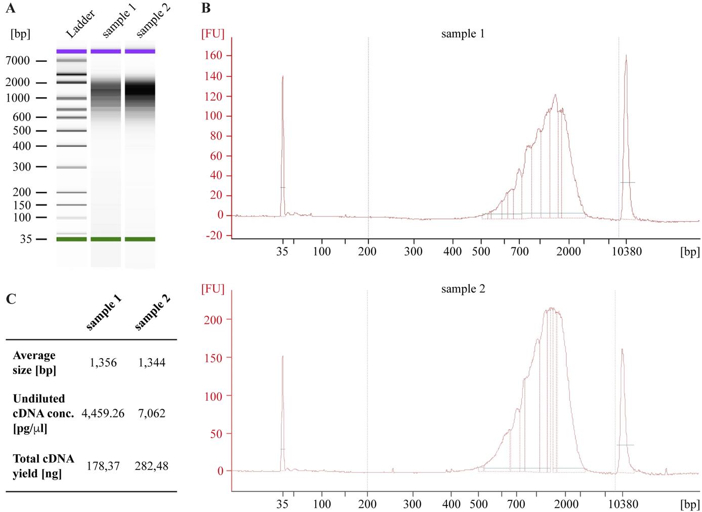
Figure 4. Representative readout from Agilent 2100 Bioanalyzer. A, B. Electrophoresis gel image (A) and electropherogram traces (B) of two amplified cDNA samples. bp, base pair; FU, fluorescence unit. C. Samples quality-control results after cDNA amplification.

The neocortical layer microdissection from the developing ferret brain shown in this protocol has been partially used and validated in the following research articles:

1. Singh et al. [17]. Gene regulatory landscape of cerebral cortex folding. Science Advances (Figure 1, panel A; Figure 2, panel A).

2. Martínez-Martínez et al. [18]. A restricted period for formation of outer subventricular zone defined by Cdh1 and Trnp1 levels. Nature Communications (Figure 5).

3. de Juan Romero et al. [19]. Discrete domains of gene expression in germinal layers distinguish the development of gyrencephaly. The EMBO Journal (Figure 1, panels A–E).

Landmarks for prospective SG and LS identification in embryonic and early postnatal ferret brains used in this protocol have been previously validated in the following research articles:

1. Borrell et al. [20]. In vivo gene delivery to the postnatal ferret cerebral cortex by DNA electroporation. Journal of Neuroscience (Figure 2; Figure 3, panels A, B; Figure 5, panels A, D; Figure 6).]

2. Reillo et al. [3]. A role for intermediate radial glia in the tangential expansion of the mammalian cerebral cortex. Cerebral Cortex (Figures 3–5).]

Cell lineage tracing, dye tracing, and tracking of radial fibers scaffold in the developing ferret caudal cortex were the techniques used for the faithful identification of these tissue landmarks.

General notes and troubleshooting

General notes

1. For obtaining the optimal cell concentration range for one reaction of Chromium Single Cell 3' (10× Genomics) experiment, 2–3 E34 ferret embryos or one P1 ferret kit are required. The recommended starting cell concentration might vary between single-cell assays.

2. By means of this protocol, the obtained cell concentration range for E34 samples is 7.3 × 10⁵–5.4 × 10⁶ cells/mL, for P1 samples from VZ is 6.4 × 10⁵–2.9 × 10⁶ cells/mL, and from OSVZ is 7.2 × 10⁵–2.6 × 10⁶ cells/mL.

3. After animal anesthesia, follow the protocol non-stop. A shorter experimental time, combined with tissue maintenance on ice, produces better outputs. The average experimental time for two researchers working together is 5 h.

4. Turn the light intensity from the dissecting scope up and down to facilitate distinguishing between the different neocortical layers.

5. During tissue dissociation, treat cells very gently to avoid cell death: finger flicker and invert the tubes gently, do not vortex the cells, make sure that the openings of the glass Pasteur pipettes are not too small, pipette slowly, and avoid forming air bubbles.

6. This protocol has been implemented to obtain a single-cell suspension from E34 or P1 ferret neocortical layers. If applied in more advanced ferret developmental stages, longer incubation time with the dissociating enzyme and larger mechanical dissociation should probably be used to counteract the stiffness caused by myelin. If, on the other hand, it is applied at earlier stages of development, shorter incubation time and milder mechanical dissociation might probably be recommended to avoid cell death.

Troubleshooting

Problem 1: Dissected tissue pieces have stuck to the walls or opening of the pipette tip while transferring them to the 2 mL tube.

Possible cause: The tissue has become sticky after being cut for a while.

Solution: Introduce the tip inside a Petri dish with ice-cold L-15 medium, focus on the stuck tissue with the dissecting scope, and pipette up and down with force to detach them. Do not miss sight of them to avoid losing the pieces due to their small size.

Problem 2: Single-cell suspension contains very few cells.

Possible cause: Accidental suction of the cells together with the supernatant after centrifuging.

Solution: Centrifuge the supernatants resulting from the first and second centrifugation steps at 92× g for 2 min, carefully aspirate the supernatant from both of them, resuspend the cell pellets in 40 μL of cell collection medium, and proceed to check cell concentration and viability.

Problem 3: Single-cell suspension contains clustered cells and/or debris.

Possible cause: Large size of microdissected tissue and/or low enzymatic dissociation.

Solution: Filter cell suspension again through a 40 μm pre-wet strainer to another pre-coated 2 mL tube. This second filtration can only be done once, otherwise cell membranes are compromised. In future experiments, cut the microdissected layer into smaller pieces and/or increase tube flickering during the dissociation reaction.

Acknowledgments

This work was supported by Spanish Research Agency (AEI) grants PGC2018-102172-B-I00, PID2021-125618NB-I00 and European Research Council grant UNFOLD (101118729) to V.B., who also acknowledges financial support from the AEI through the “Severo Ochoa” Programme for Centers of Excellence in R&D (CEX2021-001165-S). L.D.-V.-A. was recipient of an FPI contract from the Spanish Research Agency (AEI). This protocol was first implemented, described and validated in [8].

Competing interests

The authors declare that they have no competing interests.

Ethical considerations

All animals were treated according to Spanish and European regulations. The protocol was conducted in agreement with the Institutional Animal Care and Use Committee (IACUC) from the Spanish Council for Scientific Research (CSIC). The experimental protocol was performed at Instituto de Neurociencias on healthy ferret embryos or postnatal kits (Mustela putorius furo). Pregnant sable ferrets were housed at the Animal Research Facility (SEA) of the Miguel Hernández University (UMH), where specialized and accredited personnel were responsible for their wellbeing. They were kept in a 12/12 h light/dark cycle with standard chow and water freely accessible.

References

1. Fietz, S. A., Kelava, I., Vogt, J., Wilsch-Bräuninger, M., Stenzel, D., Fish, J. L., Corbeil, D., Riehn, A., Distler, W., Nitsch, R., et al. (2010). OSVZ progenitors of human and ferret neocortex are epithelial-like and expand by integrin signaling. Nat Neurosci. 13(6): 690–699.
2. Hansen, D. V., Lui, J. H., Parker, P. R. L. and Kriegstein, A. R. (2010). Neurogenic radial glia in the outer subventricular zone of human neocortex. Nature. 464(7288): 554–561.
3. Reillo, I., de Juan Romero, C., García-Cabezas, M. Ã. and Borrell, V. (2011). A Role for Intermediate Radial Glia in the Tangential Expansion of the Mammalian Cerebral Cortex. Cereb Cortex. 21(7): 1674–1694.
4. Shitamukai, A., Konno, D. and Matsuzaki, F. (2011). Oblique Radial Glial Divisions in the Developing Mouse Neocortex Induce Self-Renewing Progenitors outside the Germinal Zone That Resemble Primate Outer Subventricular Zone Progenitors. J Neurosci. 31(10): 3683–3695.
5. Wang, X., Tsai, J. W., LaMonica, B. and Kriegstein, A. R. (2011). A new subtype of progenitor cell in the mouse embryonic neocortex. Nat Neurosci. 14(5): 555–561.
6. Nowakowski, T. J., Pollen, A. A., Sandoval-Espinosa, C. and Kriegstein, A. R. (2016). Transformation of the Radial Glia Scaffold Demarcates Two Stages of Human Cerebral Cortex Development. Neuron. 91(6): 1219–1227.
7. Bilgic, M., Wu, Q., Suetsugu, T., Shitamukai, A., Tsunekawa, Y., Shimogori, T., Kadota, M., Nishimura, O., Kuraku, S., Kiyonari, H., et al. (2023). Truncated radial glia as a common precursor in the late corticogenesis of gyrencephalic mammals. eLife. 12: e91406.
8. Del-Valle-Anton, L., Amin, S., Cimino, D., Neuhaus, F., Dvoretskova, E., Fernández, V., Babal, Y. K., Garcia-Frigola, C., Prieto-Colomina, A., Murcia-Ramón, R., et al. (2024). Multiple parallel cell lineages in the developing mammalian cerebral cortex. Sci Adv. 10(13): eadn9998.
9. Betizeau, M., Cortay, V., Patti, D., Pfister, S., Gautier, E., Bellemin-Ménard, A., Afanassieff, M., Huissoud, C., Douglas, R. J., Kennedy, H., et al. (2013). Precursor Diversity and Complexity of Lineage Relationships in the Outer Subventricular Zone of the Primate. Neuron. 80(2): 442–457.
10. Pilz, G. A., Shitamukai, A., Reillo, I., Pacary, E., Schwausch, J., Stahl, R., Ninkovic, J., Snippert, H. J., Clevers, H., Godinho, L., et al. (2013). Amplification of progenitors in the mammalian telencephalon includes a new radial glial cell type. Nat Commun. 4(1): 2125.
11. Kalebic, N., Gilardi, C., Stepien, B., Wilsch-Bräuninger, M., Long, K. R., Namba, T., Florio, M., Langen, B., Lombardot, B., Shevchenko, A., et al. (2019). Neocortical Expansion Due to Increased Proliferation of Basal Progenitors Is Linked to Changes in Their Morphology. Cell Stem Cell. 24(4): 535–550.e9.
12. Pollen, A. A., Nowakowski, T. J., Chen, J., Retallack, H., Sandoval-Espinosa, C., Nicholas, C. R., Shuga, J., Liu, S. J., Oldham, M. C., Diaz, A., et al. (2015). Molecular Identity of Human Outer Radial Glia during Cortical Development. Cell. 163(1): 55–67.
13. Thomsen, E. R., Mich, J. K., Yao, Z., Hodge, R. D., Doyle, A. M., Jang, S., Shehata, S. I., Nelson, A. M., Shapovalova, N. V., Levi, B. P., et al. (2015). Fixed single-cell transcriptomic characterization of human radial glial diversity. Nat Methods. 13(1): 87–93.
14. Matsumoto, N., Tanaka, S., Horiike, T., Shinmyo, Y. and Kawasaki, H. (2020). A discrete subtype of neural progenitor crucial for cortical folding in the gyrencephalic mammalian brain. eLife. 9: e54873.
15. Li, Z., Tyler, W. A., Zeldich, E., Santpere Baró, G., Okamoto, M., Gao, T., Li, M., Sestan, N. and Haydar, T. F. (2020). Transcriptional priming as a conserved mechanism of lineage diversification in the developing mouse and human neocortex. Sci Adv. 6(45): eabd2068.
16. Del-Valle-Anton, L. and Borrell, V. (2022). Folding brains: from development to disease modeling. Physiol Rev. 102(2): 511–550.
17. Singh, A., Del-Valle-Anton, L., de Juan Romero, C., Zhang, Z., Ortuño, E. F., Mahesh, A., Espinós, A., Soler, R., Cárdenas, A., Fernández, V., et al. (2024). Gene regulatory landscape of cerebral cortex folding. Sci Adv. 10(23): eadn1640.
18. Martínez-Martínez, M. Ã., De Juan Romero, C., Fernández, V., Cárdenas, A., Götz, M. and Borrell, V. (2016). A restricted period for formation of outer subventricular zone defined by Cdh1 and Trnp1 levels. Nat Commun. 7(1): 11812.
19. de Juan Romero, C., Bruder, C., Tomasello, U., Sanz‐Anquela, J. M. and Borrell, V. (2015). Discrete domains of gene expression in germinal layers distinguish the development of gyrencephaly. EMBO J. 34(14): 1859–1874.
20. Borrell, V. (2010). In vivo gene delivery to the postnatal ferret cerebral cortex by DNA electroporation. J Neurosci Methods. 186(2): 186–195.