- Protocols

- Articles and Issues
- For Authors
- About
- Become a Reviewer

An Optimized P. berghei Liver Stage–HepG2 Infection Model for Simultaneous Quantitative Bioimaging of Host and Parasite Nascent Proteomes
Published: Vol 14, Iss 5, Mar 5, 2024 DOI: 10.21769/BioProtoc.4952 Views: 1926
Reviewed by: Clara Morral MartinezRaniki KumariAnonymous reviewer(s)
Original research article
The authors used this protocol in:
Nov 2023
Advertisement


Protocol Collections
Comprehensive collections of detailed, peer-reviewed protocols focusing on specific topics


Related protocols
Abstract
The Plasmodium parasites that cause malaria undergo an obligate, asymptomatic developmental stage in the host liver before initiating the symptomatic blood-stage infection. The parasite liver stage is a key intervention point for antimalarial chemoprophylaxis: successful targeting of liver-stage parasites prevents disease development in individuals and can help to reduce parasite transmission in populations, as the gametocyte forms that transmit infection to mosquitos are exclusively found in the blood stage. Antimalarial drugs that can target multiple parasite stages are thus highly desirable, and one emerging cellular target for such multistage active compounds is the process of protein synthesis or translation. Quantitative study of liver stage translation, and thus mechanistic evaluation of translation inhibitors against liver stage parasites, is not amenable to the methods allowing quantification of asexual blood stage translation, such as radiolabeled amino acid incorporation or lysate-based translation of reporter transcripts. Here, we present a method using o-propargyl puromycin (OPP) labeling of host and parasite nascent proteomes in the P. berghei-HepG2 infection model, followed by automated confocal image acquisition and computational separation of P. berghei vs. H. sapiens nascent proteome signals to allow simultaneous readout of the effects of translation inhibitors on both host and parasite. This protocol details our HepG2 cell culture and infected monolayer handling optimized for microscopy, our OPP labeling workflow, and our approach to automated confocal imaging, image processing, and data analysis.
Key features
• Uses the o-propargyl puromycin labeling technique developed by Liu et al. to quantitatively analyze protein synthesis in Plasmodium berghei liver-stage parasites in actively translating hepatoma cells.
• This quantitative approach should be adaptable for other puromycin-sensitive intracellular pathogens residing in actively translating host cells.
• The P. berghei–infected HepG2 recovery and reseeding protocol presented here is of use in applications beyond nascent proteome labeling and quantification.
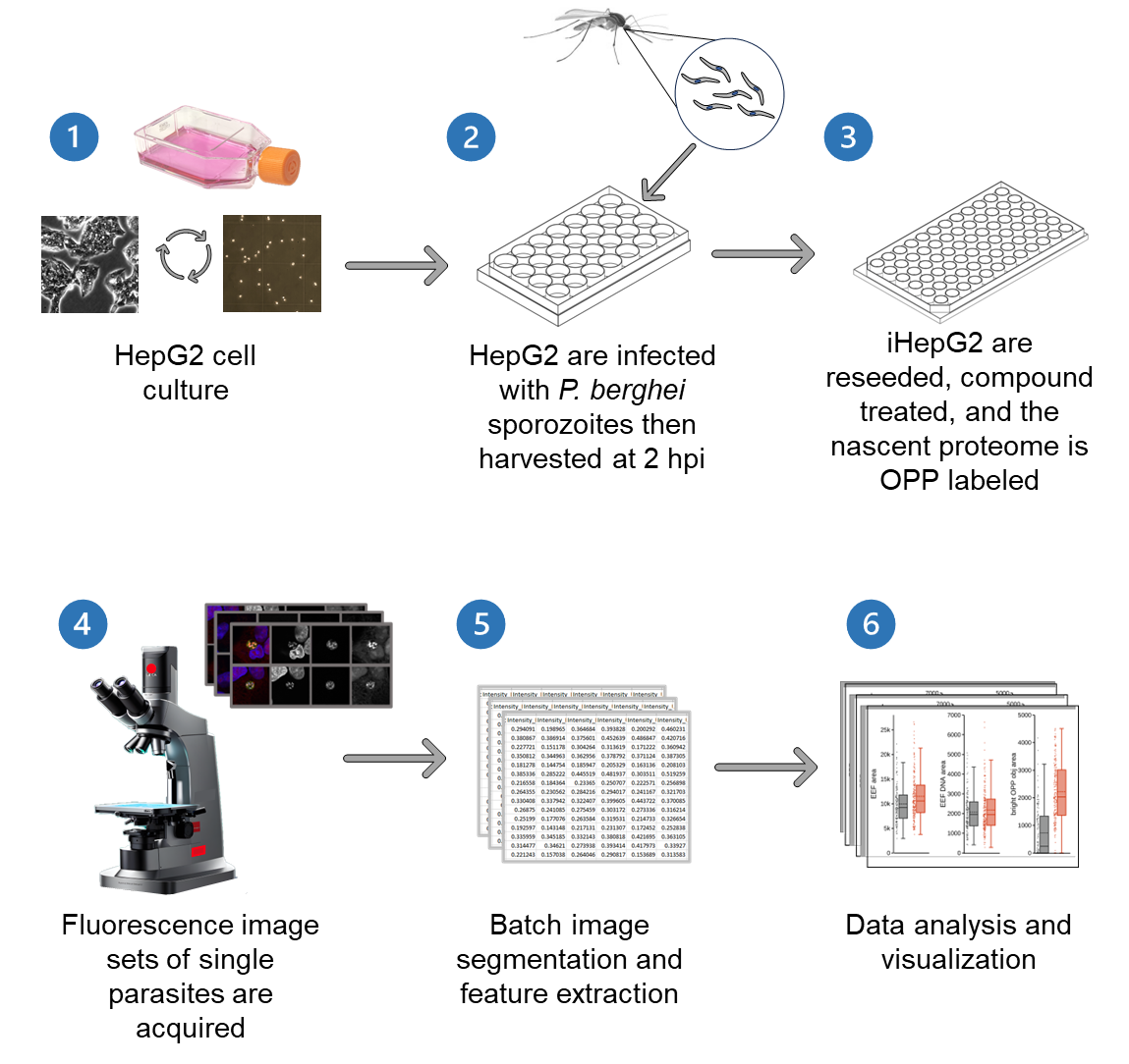
Graphical overview
Background
Plasmodium parasites, the causative agents of malaria, have a complex lifecycle spanning both mosquito and human hosts. The first obligate step for parasite development in humans occurs in the liver following the introduction of motile parasites forms, called sporozoites, via an anopheline mosquito bite. Here, the liver-stage parasites, or exoerythrocytic forms (EEFs), undergo an extensive growth and replication process entirely within a parasitophorous vacuole in the cytoplasm of a hepatocyte; a single sporozoite will result in the formation of thousands of hepatic merozoites, which initiate the blood stage of infection [1]. While the continuous asexual replication cycles of blood-stage parasites can give rise to the signs and symptoms of malaria, the liver stage is asymptomatic and a key target for both vaccination strategies and chemoprophylaxis. The most widely used model species for studying the Plasmodium liver stage is P. berghei, a rodent malaria parasite that is capable of invading and growing in a variety of cell lines, including human hepatoma cell lines, during its liver-stage development [2,3]. Several immortalized cell lines are in regular use today, including HepG2 (human hepatoma), Huh-7 (human hepatoma), and HeLa (human cervical adenocarcinoma). Hepatocytes are highly specialized, polarized epithelial cells making up the liver parenchyma, and HepG2 are unique amongst the cell lines used for P. berghei liver-stage infections in their substantial maintenance of hepatic polarity, thus providing the closest in vitro cellular environment to that of the native host hepatocytes within a mammalian liver [4,5]. Hepatocytes in the liver are arranged in chords within hexagonal lobules in an architecture where each hepatocyte has direct basal surface contact with blood flowing through the fenestrated sinusoidal endothelium, while its multiple apical surfaces form the lumina into which bile is secreted at lateral points of contact with other hepatocytes [4,5]. The regenerative capacity of the liver relies on the ability of quiescent hepatocytes to reenter the cell cycle and divide, and the organizing principle that keeps the architecture of the chords intact relies on precise alignment of the daughter cells along the sinusoid [6]. These structural and functional particularities of the native hepatocyte environment have consequences for the in vitro growth of polarized HepG2 cells, which have a reputation for forming 3-dimensional layers or clumps in the absence of the liver architecture, which can hinder quantitative bioimaging in the P. berghei–HepG2 infection model. Careful attention to HepG2 culture and passage conditions can minimize this, allowing quantitative bioimaging of both host and parasite characteristics like translational output, which we present here.
Core cellular processes are somewhat difficult to study in Plasmodium liver stages. Protocols for routine isolation of EEFs have not been reported, so signals from the parasite must be separated from those of both infected and uninfected hepatocytes in the culture. While quantitative translation assays exist for Plasmodium blood-stage parasites [7–9], to our knowledge this is the first protocol for direct quantification of liver-stage translation in single cells and populations in the P. berghei–HepG2 infection model [10,11]. This assay relies on the use of the modified puromycin analogue, o-propargyl puromycin (OPP) [12], to label the HepG2 and P. berghei nascent proteomes during a 30 min window, followed by fixation, click chemistry–based attachment of a fluorophore to the OPP-labeled nascent polypeptides, and immunolabeling of the parasites, followed by confocal imaging, batch image segmentation and feature extraction to computationally separate HepG2 and parasite signals, and data analysis.
Materials and reagents
Biological materials
Plasmodium berghei ANKA (676 m1cl1)–infected Anopheles stephensi mosquitos (University of Georgia SporoCore)
HepG2 human hepatoma cell line (ATCC STR profiling-verified)
Reagents
DMEM (Gibco, catalog number: 10313-021)
Pen Strep (Gibco, catalog number: 15140-122)
Heat inactivated fetal bovine serum (FBS) (Gibco, catalog number: 16140-071)
GlutaMAX (Gibco, catalog number: 35050-061)
TrypLE Express (Gibco, catalog number: 12605-028)
Dulbecco’s PBS (DPBS) (Sigma, catalog number: D8537)
PBS (Sigma, catalog number: P3813)
Triton X-100 (Sigma, catalog number: T9284)
Paraformaldehyde (PFA) solution, 4% in PBS (Thermo Scientific, catalog number: 30525-89-4)
Penicillin Streptomycin Neomycin (PSN) (100×) (Gibco, catalog number:15640-055)
Kanamycin sulfate (Corning, catalog number: 30-006-CF)
Amphotericin B (Gibco, catalog number: 15290-026)
Gentamycin (Gibco, catalog number: 15750-060)
DMSO (Sigma, catalog number: D2650)
Anisomycin (EMD Millipore-Sigma, catalog number: 176880)
O-propargyl-puromycin (OPP) (Invitrogen, catalog number: 10459)
O-propargyl-puromycin (OPP) [Vector labs (formerly Click Chemistry Tools), catalog number: CCT-1407-5]
Click-iT® Plus Alexa Fluor® 555 picolyl azide toolkit (Invitrogen, catalog number: C10642)
Click-&-Go® Plus 555 Imaging kit (Vector labs, catalog number: CCT-1317)
Bovine serum albumin (BSA) (Fisher Bioreagents, catalog number: 9048-46-8)
Mouse anti-PbHsp70 primary antibody [13]
Donkey anti-mouse Alexa Fluor® 488 (Invitrogen, catalog number: A21202)
Hoechst 33342 (10 mg/mL) (Thermo Scientific, catalog number: 62249)
70% ethanol
Laboratory supplies
25 cm2 cell culture flask (Corning, catalog number: 430168)
75 cm2 cell culture flask (Corning, catalog number: 430720U)
Cell strainer, 40 μm nylon (Corning, catalog number: 431750)
Cell strainer, 100 µm nylon (Corning, catalog number: 431752)
0.22 µm filters (Millex, catalog number: SLGV004SL)
0.20 µm filters (Corning, catalog number: 431229)
1 mL syringes (BD, catalog number: 309659)
10 mL syringes (BD, catalog number: 302995)
1 mL syringes with hypodermic needle (BD, catalog number: 309626)
50 mL conical tubes (Corning, catalog number: 430828)
24-well cell culture plate (Corning, catalog number: 3524)
12 mm round coverslips, 1.5 thickness (Azer, catalog number: ES0117520)
Fluoromount-G (SouthernBiotech, catalog number: 0100-01)
96-well µClear cell culture plate (Greiner bio-one, catalog number: 655098)
96-well round bottom plate (Corning, catalog number: 3799)
5 mL serological pipettes (Corning, catalog number: 4487)
10 mL serological pipettes (Corning, catalog number: 4488)
25 mL serological pipettes (Corning, catalog number: 4489)
Reagent reservoirs (Eppendorf, catalog number: 022265806)
Live insect forceps (FST, catalog number: 26029-10)
Dumont #5/45 coverslip forceps (FST, catalog number: 11251-33)
6-well plate (Corning, catalog number: 351146)
Neubauer chamber (Brand GMBH, catalog number: 717805)
Pestle (Fisherbrand, catalog number: 12-141-363)
Multichannel racked pipette tips, 1,200 µL (Rainin, catalog number: 17002921)
Multichannel racked pipette tips, 300 µL (Rainin, catalog number: 30389255)
P1000 barrier pipette tips (Thermo Scientific, catalog number: 2079)
Microscope slides 75 × 25 × 1 mm (VWR, catalog number: 16004-368)
1.7 mL snap top tubes (Axygen, catalog number: MCT-175-A)
Kimwipes
Paper towels
Ice bucket
Solutions
Complete DMEM (cDMEM) (see Recipes)
Infection DMEM (iDMEM) (see Recipes)
DMSO control treatment (see Recipes)
Anisomycin control treatment (see Recipes)
0.5% Triton-X (see Recipes)
Blocking solution (see Recipes)
Click-iT® Plus Master Mix (see Recipes)
1° (primary) antibody solution (see Recipes)
2° (secondary) antibody solution (see Recipes)
Recipes
Complete DMEM (cDMEM)
Reagent Final concentration Quantity or Volume DMEM 88% (v/v) 440 mL FBS
Pen Strep
GlutaMAX
10% (v/v)
1% (v/v)
1% (v/v)
50 mL
5 mL
5 mL
Total n/a 500 mL Infection DMEM (iDMEM)
Reagent Final concentration Quantity or Volume cDMEM 97.5% (v/v) 97.5 mL PSN
Kanamycin sulfate
Amphotericin B
Gentamycin
1% (v/v)
1% (v/v)
0.33% (v/v)
0.1% (v/v)
1 mL
1 mL
334 µL
100 µL
Total n/a 100 mL DMSO control treatment
Reagent Final concentration Quantity or Volume iDMEM n/a 1,998 µL DMSO 0.1% (v/v) 2 µL Total n/a 2,000 µL Anisomycin control treatment
Reagent Final concentration Quantity or Volume iDMEM n/a 1,998 µL 10 mM stock of anisomycin 0.1% (v/v) 2 µL Total n/a 2,000 µL 0.5% Triton-X
Reagent Final concentration Quantity or Volume PBS n/a 4,750 µL 10% Triton X-100 0.5% (v/v) 250 µL Total (optional) n/a 5 mL Blocking solution (2% BSA in PBS)
Reagent Final concentration Quantity or Volume BSA 2% (w/v) 1 g PBS n/a 50 mL Total n/a 50 mL Click iT® Plus Master Mix
Note: All reagents should be prepared and stored in accordance with manufacturer’s specifications. Components should be brought to room temperature before making master mix. Each master mix should be prepared fresh and used within 15 min. Each component of the master mix should be added in the order listed. The CuSO4 and copper protectant mix should be combined separately before addition to the master mix; these components are stored separately to allow you to change the concentration of copper catalyst in the reaction master mix by adjusting the ratio of CuSO4 to copper protectant buffer. We have found that a 1:4 ratio of copper–copper protectant provides nearly identical signal compared to those of higher ratios. The total volume reported here is designed for a 96-well plate (32 wells at 27 µL each) with ample dead volume.
Reagent Final concentration Quantity or Volume Molecular grade H2O 78.3% (v/v) 783 µL 10× Click-iT® reaction buffer
500 µM Alexa Fluor® PCA solution
CuSO4-copper protectant mix
1×x Click-iT® buffer additive
8.7% (v/v)
1% (v/v)
2% (v/v)
10% (v/v)
87 µL
10 µL
20 µL
100 µL
Total (optional) n/a 1,000 µL 1° antibody solution
Note: Anti-PbHSP70 working dilution will depend on antibody concentration; the dilution given is for an unpurified batch produced from the 2E6 hybridoma in the Hanson lab. Antibody solutions are filtered using 0.20–0.22 µm filters before use.
Reagent Final concentration Quantity or Volume Blocking solution n/a 1,592 µL Mouse anti-PbHSP70 1:200 (v/v) 8 µL Total (optional) n/a 1,600 µL 2° antibody solution
Note: Antibody solutions are filtered using 0.20–0.22 µm filters before use.
Reagent Final concentration Quantity or Volume Blocking solution n/a 1595.2 µL Donkey anti-mouse Alexa Fluor® 488
Hoechst 33342 (10mg/mL)
1:500 (v/v)
1:1,000 (v/v)
3.2 µL
1.6 µL
Total (optional) n/a 1,600 µL
Equipment
SP8 confocal microscope (Leica, model: TCS SP8)
Dissecting stereoscope (Leica, model: S4E)
Inverted phase contrast microscope (Zeiss, model: Invertoskop 40 C)
Inverted fluorescence microscope (Leica, model: DM IL LED)
Fluorescence light source (Leica, model: EL6000)
Water bath (Thermo, model: 280 series)
CO2 incubator (Thermo, model: Napco Series 8000 WJ)
Biological safety cabinet (LABGARD, model: Class II, Type A2)
Centrifuge with swinging bucket rotor (Thermo, model: Sorval ST 40R, TX-750 rotor)
Titanium liquid removal chambers for swinging bucket rotor centrifuge (custom fabrication by Autotiv)
Small bench centrifuge (Eppendorf, model: 5415D)
Multichannel pipette 300 µL LTS (Rainin, model: E4 XLS)
Multichannel pipette 1200 µL LTS (Rainin, model: E4 XLS)
Software and datasets
LAS AF 3 (Leica)
MatrixScreener (HCS A Developer Full with CAM Leica)
CellProfiler (v2.1.1 rev6c2d896, 7/25/2014), used for image segmentation and feature extraction
CellProfiler (v2.0.11710, 01/24/2014), used for online image segmentation and parasite ID during automated confocal feedback microscopy (ACFM)
KNIME version 4.7.7 and earlier v4 releases (01/20/2022), used for data analysis
Procedure
HepG2 cell culture optimized for imaging
Note: All steps involving live HepG2 cells are performed in a biosafety cabinet.
Prepare cDMEM (Recipe 1).
Ensure cDMEM, DPBS, and TrypLE are at room temperature (RT).
Remove the T75 cell culture flask containing HepG2 cells from the 5% CO2, 37 ºC incubator, decant medium from the flask, and gently wash cell monolayer two times with 10 mL of DPBS.
Critical: These DPBS washes are important for the removal of residual cDMEM, which can hinder the breakdown of cell–cell junctions in the TrypLE digestion step.
Decant the second DPBS wash and add 7.5 mL of room-temperature TrypLE. Return flask to the 5% CO2, 37 ºC incubator for 10 min.
Critical: Do not disturb the flask during incubation and do not attempt to disrupt the HepG2 monolayer by tapping the flask. It is far easier to disrupt the cell-substrate attachment than to break down the cell–cell junctions, and the latter is crucial for maintaining the cells in a monolayer.
Remove the flask and add 7.5 mL of cDMEM to the TrypLE using a serological pipette, repeatedly washing the cell monolayer using the shearing forces of the dispensed liquid to dislodge the attached cells and break up any connected clumps or groups of cells.
After all cells have been removed from the plastic substrate, aspirate the cell suspension using a serological pipette and dispense through a sterile Ø40 µm filter into a 50 mL conical tube.
Critical: Filtering removes any large clumps or sheets of cells that could interfere with monolayer formation in continuous culture or when seeding cells for infection.
Centrifuge the filtered cell suspension at 315× g (1,200 rpm) for 5 min.
Discard supernatant and resuspend the pellet with 900 µL of cDMEM using p1000 with a filtered tip (>30 up-down cycles).
Add 9.1 mL of cDMEM to resuspended cells and invert several times to thoroughly mix cell suspension.
Prepare a 1:5 dilution of cell suspension by removing 10 µL of cell suspension and adding it to 40 µL of cDMEM in a snap top tube.
Place the bulk cell suspension at 4 °C while counting the cell suspension dilution.
Dispense 10 µL of the 1:5 dilution of the cell suspension into a Neubauer chamber and count all four outer quadrants (see illustration). Using the average of these four quadrants, calculate the concentration of cells in suspension using the formula shown in figure 1.
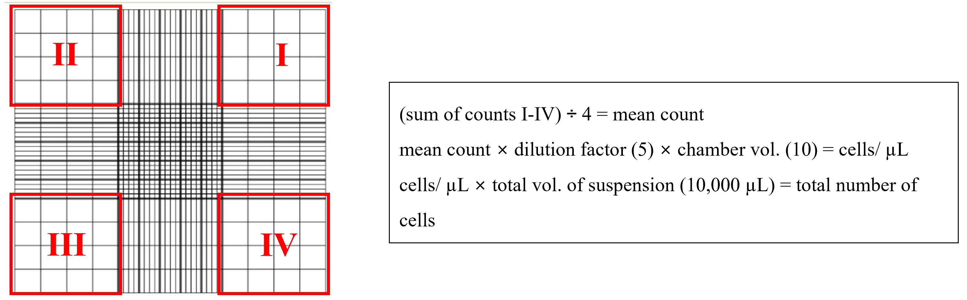
Figure 1. Counting chamber example formula. Illustration of counting chamber showing four quadrants used for counting with an explanation for calculating the cells/µL and the total number of cells in suspension.Prepare cell suspensions at the desired seeding concentration for continued propagation of cells (see Table 1).
Table 1. Schedule for HepG2 cell passage. We always seed a backup flask during each cell passage in case of delayed mosquito arrival, contamination of the primary flask during passage, etc. We maintain each backup flask in the incubator through two passages of the main flask. We use HepG2 cells in assays from p2 through p15. M = million.
Monday Tuesday Wednesday Thursday Friday T-75 primary flask Seed 2.4 m cells for Thursday split Seed 1.8 m cells for Monday split T-25 backup flask 0.8 m cells 0.6 m cells With the remaining cell suspension, proceed to section B.
Seeding HepG2 cells for infection
Note: This protocol details the quantification of liver-stage translation and small molecule–induced translation inhibition in P. berghei–infected HepG2 cells in a 96-well plate format, but this can also be performed in a coverslip format. See general note 3 for details.
Calculate the number of cells required for experiments and prepare an appropriately diluted seeding solution in cDMEM. To seed a 24-well plate with 150,000 HepG2 per well in a volume of 500 µL [(24 wells + 1 well dead volume) × 150,000 cells] = 3,750,000 cells to be suspended in (25 wells × 500 µL) = 12.5 mL of seeding suspension.
Note: HepG2 cells should never be a limiting reagent. Since sporozoite yield cannot be fully predicted in advance of the dissection, we always seed more HepG2 wells than we predict we will need.
Invert tube containing the cell suspension several times to ensure it is properly mixed.
Dispense 500 µL of cell suspension to each well of the 24-well plate.
Carefully redistribute cells within each well by tracing the figure ∞ 10–13 times, rotate the plate 180°, and trace the figure ∞ an additional 10–13 times.
Critical: An uneven cell distribution can affect invasion success and hinder imaging.
Note: Inspect the cell distribution of several wells using a microscope at a low magnification. You can get a good idea of the cell distribution by adjusting the focal plane and moving through the well contents in the Z-axis. If the cells are not evenly distributed upon visual inspection, repeat figure ∞ steps again.
Return plates to the incubator for 20–24 h before the anticipated time of infection the next day.
P. berghei sporozoite infection of HepG2 cells
Note: Up until the point of HepG2 infection, it is crucial to keep sporozoites on ice whenever a solution is not being directly handled. As before, all steps involving live HepG2 cells are performed in a biosafety cabinet. For more information regarding mosquito dissection and sporozoite isolation, see general note 1.
Visually inspect the cells seeded the previous day to ensure that they are adherent and growing normally and that no wells are contaminated.
Prepare iDMEM (Recipe 2).
Collect the mosquitos that are to be dissected into a 50 mL conical tube, cold-anesthetize them for 5 min at -20 °C, and then remove and place the tube of mosquitos horizontally on ice in a benchtop ice bucket.
Critical: Prolonged exposure to -20 °C or exposure to lower temperatures can affect sporozoite viability.
Using insect forceps, carefully transfer ~50 mosquitos into a Ø100 µm cell strainer. Using a 6-well plate as a wash station, immerse them into a well containing 70% ethanol (5–6 s), blot excess ethanol on a paper towel, then rinse in HBSS by immersion into two successive wells.
Note: This washing procedure helps to reduce contamination by the mosquito-surface microbiome.
Transfer the mosquitos into a large drop of DMEM on a glass microscope slide and immobilize a mosquito by gently pressing down on the thorax with the blunt side of a hypodermic needle using the non-dominant hand. Using another needle in the dominant hand, gently pull the mosquito head (with salivary glands attached) away from the thorax and cleave the salivary glands from the head with the sharp edge of the needle.
Note: If the salivary glands do not separate with the head, applying gentle pressure to the thorax will allow gland removal from the opening of the thorax. See general note 1 for additional resources and instructional guides for mosquito dissection and anatomy.
Transfer each set of glands to a 1.6 mL snap top tube containing 100 µL of DMEM, which is kept on ice.
Note: Cold anesthetized mosquitos and salivary glands should be kept on ice throughout the dissection procedure, and total time spent dissecting should be minimized to ensure sporozoite viability.
Release sporozoites by grinding the isolated salivary glands for 15–30 s using a sterile pestle and wash the walls of the tube and the pestle with additional DMEM, keeping the total volume of DMEM below 1 mL.
Note: The mosquito salivary glands must be disrupted to release sporozoites into the media. If this step is not done properly, the sporozoites will remain in the salivary glands and will be removed by filtering in the next step. For additional resources and alternative methods for releasing sporozoites from the salivary gland see general note 1.
Pass sporozoite material through a Ø100 µm cell strainer into a 50 mL conical tube. Using a micropipette, very gently recover any remaining medium from the bottom of the strainer and add it to the collection.
Centrifuge the sporozoite solution at 100× g for 30 s to ensure that all liquid is collected and transfer it into a 1.6 mL snap top tube.
Prepare a 1:5 counting dilution, mixing the sporozoite solution vigorously by manually flicking the tube; then, remove 10 µL of sporozoite solution and add it to 40 µL of DMEM. Mix this solution by vigorous pipetting using the same tip that transferred the sporozoites. Then, transfer 10 µL of this solution into a Neubauer chamber, place the chamber into a humidified, foil-covered dish, and allow the sporozoites to settle for 8 min; then, count the sporozoites as in Figure 1.
Note: If the sporozoite count in a single 4 × 4 counting grid exceeds 100 sporozoites, it is preferable to further dilute the counting dilution and then repeat the steps here and recount (e.g., adding 40 µL of medium to the remaining 40 µL of counting solution would yield a 1:10 dilution).
Based on the total number of sporozoites recovered, calculate the number of wells that can be infected with 100,000 sporozoites per well.
Dilute concentrated sporozoites into iDMEM to infect each well using a total volume of 300 µL. Assuming a recovery of 1 million sporozoites in a total volume of 800 µL, 10 wells could be infected. To reach a final volume of 3 mL, 800 µL containing 1 × 10⁶ sporozoites would be added to 2.2 mL of iDMEM.
Remove the HepG2 cell plate from the incubator, carefully aspirate the cDMEM from each well, and replace with 300 µL of the sporozoite suspension prepared in the previous step.
Centrifuge plate at 2,000× g (3,000 rpm) for 5 min and return the plate to the 5% CO2, 37 °C incubator for 2 h.
Note: Record the exact time when the plates are returned to the incubator, as this will correspond to t0, and future steps will take place at a set number of hours post-infection (hpi).
At 2 hpi, remove the plate from the incubator, extract the iDMEM from each well using a p1000 filter-tipped micropipette, and add 1,000 µL of room-temperature DPBS.
Remove dPBS from each well and replace it with 200 µL of TrypLE. Return to the 5% CO2, 37 °C incubator for 10 min.
Transfer plate from incubator to sterile hood and add 200 µL of fresh iDMEM to each well containing TrypLE.
Using a filter-tipped P1000 with volume set to 300 µL, repeatedly pipette up and down across the entire bottom of the well, using fluid force to dislodge the infected HepG2 (iHepG2) from the substrate into a single-cell suspension. Then, transfer the entire 400 µL into a 50 mL collection tube and immediately add 200 µL of iDMEM to the well.
Once all wells have been processed, inspect the plate well by well to ensure that all iHepG2 from the monolayer were successfully harvested.
Critical: Once exposed to the sporozoite solution, HepG2 are even stickier than normal, and an inexperienced investigator may find that many cells remain in each well. If so, repeat well washing steps to detach cells by fluid force with a micropipette and add to the collection tube.
Using a serological pipette, transfer the suspended iHepG2 through a Ø40 µm strainer into a 50 mL conical tube to remove any large cell clumps and mosquito debris.
Centrifuge at 315× g (1,200 RPM) for 5 min.
Discard supernatant and resuspend the pellet with 900 µL of iDMEM using a p1000 with a filtered tip (at least 50 up and down cycles, as infected HepG2 are harder to separate compared with uninfected cells).
Add iDMEM to a final volume equal to 1 mL × the number of wells trypsinized; so, with 10 wells harvested, add 9.1 mL.
Remove a small sample of infected cell suspension for counting and place the bulk cell suspension at 4 °C while counting.
Dispense 10 µL of the undiluted infected cell suspension into a Neubauer chamber and count infected cells as previously described (Figure 1).
Based on the number of iHepG2 cells recovered, calculate the number of wells and plates needed for reseeding and prepare iHepG2 cell suspension for seeding. Each well of a 96-well plate will be seeded with 25,000 iHepG2 in a total volume of 200 µL per well. Typical iHepG2 recovery is ~200,000 cells per well of a 24-well plate, so the concentration will be 200 cells/µL. For this example, we will seed one 96-well plate for imaging. Due to steric hindrance from the microscope objective used, we work only in the inner 32 wells of each plate, and for each plate to be seeded with an electronic 8-channel pipette, a dead volume corresponding to one well is added. For this, (33 wells × 25,000 cells) = 825,000 iHepG2 are required in a total volume of 6.6 mL; 825,000 iHepG2/200 = 4.13 mL of iHepG2 suspension is needed, which will be added to 2.35 mL of iDMEM.
Transfer the iHepG2 seeding suspension into a sterile reagent reservoir and use a serological pipette to thoroughly mix the solution by up and down pipetting 3–5 times.
Using a p1200 8-channel electronic pipette, dispense 200 µL of iHepG2 suspension into the desired number of wells.
Let cells settle at RT for 10 min shielded from the light and then place plates in 5% CO2, 37 °C incubator.
Compound treatments, OPP labeling, and fixation
Note: We developed this protocol to quantify the activity of translation inhibitors, which is compared to DMSO controls (test compound vehicle) and known active controls such as anisomycin. The protocol steps listed below are a detailed demonstration of one assay modality—the acute pretreatment format, where test compounds and controls are applied to iHepG2 from 24–28 hpi; during the last 30 min of the treatment period, OPP is added to each well and the nascent proteome is labeled in the continued presence of treatment compounds. This assay can be modified in several ways; see general note 2.
Prepare test compound treatments, DMSO control treatments, and anisomycin control treatment, transferring them to a 96-well round-bottom plate matching the desired assay plate layout, if not already in this format. Do this in sufficient time to ensure that solutions are at RT at 24 hpi.
Critical: Regardless of compound concentration being tested, the concentration of the DMSO solvent must be identical between treatments, positive controls, and DMSO controls. DMSO concentration in every well should be 0.1% (see Recipes 3–4).
Note: We include four DMSO control wells and one anisomycin active control well on each plate to ensure robust normalization during later analysis.
At 24 hpi, carefully aspirate all iDMEM from each well using a p300 multichannel pipette and replace it with 200 µL of treatment-containing medium from the compound plate prepared in step D1. Then return assay plate to 5% CO2, 37 °C incubator.
At 26.5 hpi, prepare 250 µL of a 20× (400 µM) OPP solution in iDMEM, transfer 30 µL to wells A1–A8 of a round-bottom 96-well plate, and prewarm it in the 5% CO2, 37 °C incubator.
Critical: OPP labeling needs to occur at 37 °C for efficient and effective labeling. Ensure that samples and OPP labeling media are properly warmed to 37 °C before labeling.
Note: We have used two different sources of OPP (see reagents list) and detected no difference in labeling.
At 27 hpi, remove 105 µL of treatment media from each well using a multichannel pipette, leaving 95 µL in each well.
Return the treatment plate with reduced treatment volumes to the incubator for 30 min.
Note: Reducing the medium volume and returning samples to the incubator for 30 min in advance of OPP addition helps to ensure the temperature of the samples is 37 °C when OPP is added.
At 27.5 hpi, transfer the sample plate and the plate containing OPP-labeling solution to the biosafety cabinet. Using a multichannel pipette, dispense 5 µL of 20× OPP solution to each well.
Note: This step should be performed quickly to prevent everything from cooling of the medium.
Gently swirl the plate 5–6 times, quickly return the plate to the incubator, and start a 30 min timer.
After 30 min (at ~28 hpi), remove the plate from the incubator, take off the lid, and place the plate face-down in a swinging bucket rotor liquid removal chamber. Remove media by centrifuging plate at 79× g for 15 s.
Critical: Swinging bucket rotor liquid removal chambers need to be manufactured in weight-matched pairs and, in the case of handling a single plate, the centrifuge should be balanced by adding the equivalent volume (here, 3.2 mL) of water to the other liquid removal chamber and topping it with a matching empty 96-well plate.
Fix cells by dispensing 100 µL of 4% PFA in PBS that has been prewarmed to RT; allow samples to fix for 15 min at RT.
After fixation, flick out the PFA and wash the samples with 200 µL of PBS three times.
Seal plates in parafilm and store at 4 °C overnight.
Note: It is also possible to proceed directly to permeabilization and fluorophore addition by click chemistry. We have successfully performed click reactions on samples that have been stored for several days at 4 °C without reducing the fluorescence signal intensity or fidelity of the click reaction, but samples should be processed in a timely manner to avoid sample degradation. If plates are being stored at 4 °C for several days, the addition of 0.05% sodium azide in PBS helps to reduce bacterial contamination.
Permeabilization and click-chemistry fluorophore addition
Remove plate from 4 °C and allow it to warm to RT.
To permeabilize, flick out PBS and replace with 100 µL of 0.5% triton X-100 in PBS (Recipe 5) for 20 min at RT.
Note: Triton solution should be made fresh from 10% stock each time.
Flick out permeabilization solution and wash cells three times with 100 µL of PBS.
Incubate cells in 100 µL of blocking solution (Recipe 6) while click reaction master mix is prepared (minimum 5 min at RT).
Make click reaction master mix (MM) (Invitrogen click-iT® Alexa Fluor® 555 picolyl azide) according to manufacturer’s protocol. To label 32 wells with a minimum of 27 µL per well with ample dead volume, you need to prepare 1,000 µL (detailed in Recipe 7).
Critical: All components should be brought to room temperature before making MM.
Critical: When preparing the master mix, combine each component in the order listed in Recipe 7, per manufacturer’s recommendation.
Note: We have also successfully used Vector Labs Click-&-Go® Plus 555 Imaging Kit for click reactions with no detectable difference in the fluorescence labeling.
Flick out blocking solution and dispense 27 µL of click reaction to each well. Allow reaction to proceed shielded from light for 30 min at RT.
Flick out click reaction MM and wash the plate with blocking solution three times.
Using a fluorescence microscope, visually inspect each well of the clicked sample to ensure that DMSO controls are brightly labeled before proceeding to DNA or immunofluorescence labeling.
Prior to immunolabeling, block samples by incubating in blocking solution for 1 h at RT.
After blocking, flick out blocking solution, replace with 1° antibody solution (Recipe 8), and incubate at RT for 4 h shielded from light.
Remove 1° antibody solution and wash sample three times with blocking solution.
Flick out blocking solution and replace with 2° antibody and Hoechst solution (Recipe 9).
Incubate samples in 2° antibody solution for 1 h at RT shielded from light.
Remove 2° antibody solution and wash samples three times with PBS.
Proceed to image acquisition steps or seal plates with parafilm and store at 4 °C until imaging.
Note: Plates are imaged in PBS.
Image acquisition
Note: We use automated confocal feedback microscopy (ACFM) on a computer-aided microscopy-licensed Leica SP8 confocal running MatrixScreener directly interfacing with an early version of Cell Profiler (v 2.0.11710) via plugins (https://github.com/VolkerH/MatrixScreenerCellprofiler/wiki) [14]. These coordinate task control between CellProfiler and MatrixScreener to allow real-time online image segmentation of low-resolution monolayer images to identify potential parasites in the sample based on fluorescence and size properties. Coordinates for the center of each low-resolution EEF object identified are then passed from CellProfiler to MatrixScreener, which triggers a high-magnification autofocus Z-stack for each EEF object with X and Y position set by the initial center coordinates, followed by high magnification, high resolution multichannel image acquisition. This process has been described in detail in [15]. Different implementations of feedback microscopy are possible, and the process allows for collection of large, unbiased single-parasite image sets; however, many laboratories will not have access to such a setup but can still implement OPP-imaging of host and parasite nascent proteomes through conventional user-controlled image acquisition. So, we present here the critical steps in the process agnostic to the software and hardware used to control the image acquisition process. Regardless of automated or manual image acquisition, the user should be (or consult with) an experienced microscopist, capable of determining optimal image acquisition settings for their samples and system. We run ACFM imaging experiment on mounted glass coverslips, optical plastic-bottom 96- and 384-well plates, and a variety of glass-bottom imaging dishes; choices of substrate for the cell monolayer, mounting medium, etc. will all influence the choice of objective and are best determined by an experienced microscopist familiar with the options available to the user. Here, we will present an optical plastic-bottom 96-well plate sample containing test compounds, a DMSO vehicle control, and an anisomycin-treated control, which will have both HepG2 and P. berghei translation inhibited.
After securing the plate to the stage, use a 63× water objective to inspect the DMSO control samples, searching for the brightest OPP-A555 fluorescence, and manually image a few parasites to determine appropriate settings for laser power and PMT gain so that no pixels are saturated. Repeat this process to determine optimal settings for the DNA image and the EEF marker (P. berghei HSP70) image.
Note: To assess the sensitivity and specificity of OPP-A555 labeling, a control labeling experiment can be performed as described in Figure S1 of McLellan et al., 2023 for our imaging setup. The key controls needed are 1) a well that was not treated with OPP but was click-labeled and immunostained and 2) a well that was OPP-treated and click-labeled but with omission of the Alexafluor555 picolyl azide from the reaction mix.
With these settings saved, move to the anisomycin control well and verify if the EEF marker image allows easy visual identification of the parasite in images acquired with the settings saved in 1). If not, make slight adjustments to the EEF marker image acquisition settings until this is achieved and save the settings.
A naming scheme for image files must be decided prior to the beginning of image acquisition so that images can be unambiguously assigned to a particular well downstream in the data analysis process. We suggest consulting the REMBI framework [16] to identify a suitable image naming scheme that facilitates metadata capture. For manual acquisition of data in multiple wells of a 96-well plate, we would recommend Experiment#_96wpANcoordinate_YYYYMMDDimaged_Parasite#, e.g., E15_C7_20230803_P12, where the experiment number can be matched to full experimental details in a lab notebook, the well ID can be used to match the images to the treatment received in a plat map, the date of imaging ensures that appropriate control images can be easily identified without needing to resort to image-encoded metadata inspection, and assigning each of the imaged parasites an integer starting from 1 allows each image set from the well to be easily distinguished.
Images must be acquired in an unbiased manner. If manually acquiring images, do so without visualizing anything but the parasite marker, and acquire images of parasites systemically according to predefined rules that mimic a computational process, e.g., from a starting point in the upper-left corner of each well, move rightward in the sample and acquire images of the first five parasites encountered. Then, move down in the sample such that the last parasite imaged is well outside the field of view and repeat the process moving to the left. Continue until ~30 image sets are acquired.
When a parasite is encountered, use an automated focusing algorithm to determine the Z plane, if possible, or manually focus each parasite to maximize parasite area (without visual inspection of anything except the parasite marker) and then sequentially acquire each channel using the saved settings.
Iterate this process for each well on the plate.
Critical: All images that are to be directly compared should be collected from a single imaging session and have identical handling from sections A–C described above. Both biological and technical variables can contribute to experiment-to-experiment variation, and this necessitates data normalization in downstream steps. It is absolutely essential that robust DMSO control image sets are collected in each and every imaging session.
Image segmentation and feature extraction
Note: We perform batch image segmentation and feature extraction in CellProfiler. Resources for learning to use this software are available at cellprofiler.org. For each step in the analysis (termed modules in CellProfiler), there are numerous options and parameter setting adjustments that can be optimized for your needs and specific samples. Batch processing means that an identical setting throughout the Cell Profiler analysis pipeline must be used to process all samples from the same infection, which are handled identically and in parallel at every step in the process. Due to technical and biological variation between experiments, image intensities may vary between replicates and necessitate small tweaks to settings between experiments; however, the identical pipeline should always be used. For each image set analyzed in CellProfiler, a corresponding tiled image is generated, metadata-linked to the corresponding data by filename, and saved, along with all the features extracted and the specifically configured pipeline. For additional information on quantitative bioimaging please see A biologist’s guide to planning and performing quantitating bioimaging experiments [17].
Load all image sets from a single experiment into CellProfiler for batch analysis. Each image set is comprised of three images from different fluorescence channels: 1) parasite and HepG2 DNA, 2) PbHSP70-marked parasite, and 3) the OPP-A555 labeled nascent proteome of the parasite and host.
Using metadata fields encoded in the file names (described in image acquisition), define each image channel in CellProfiler.
Using the well position–encoded metadata, filter images to include only DMSO parasites, which are used to establish the settings of each analysis step of the pipeline.
First, use the Smooth module to reduce digital noise using a Gaussian filter. The typical artifact diameter setting will be dependent upon your image resolution and feature space, but for much of our ACFM imaging we use an artifact diameter of 2.
With the RescaleIntensity module, perform an intensity rescaling of the EEF image and the DNA image to improve contrast and further reduce noise for segmentation. We typically define intensity minima and maxima based on several DMSO image sets and then rescale pixels to the full intensity range. Image rescaling is needed for segmentation but not used in generating fluorescence intensity metrics.
Using the IdentifyPrimaryObjects module, identify the EEF object. We use global thresholding strategy with a two class Otsu method. We define the lower and upper bounds of the EEF object area (in pixels) based on the known size range of parasites at the given timepoint to reduce creation of artifacts. Further, we exclude any EEF objects that are touching the border of the image.
Use the ExpandOrShrinkObjects module to generate EEF objects both expanded and shrunken by several pixels.
Note: Often, EEFs are in close proximity to the HepG2 nucleus, where the most intense OPP signal in the HepG2 is usually found; these shrunken and expanded EEF objects are used in subsequent masking steps to eliminate the pixels at the host–parasite interface for accurate quantification of fluorescence from parasite vs. HepG2 nascent proteomes. See Figure 2 for example.
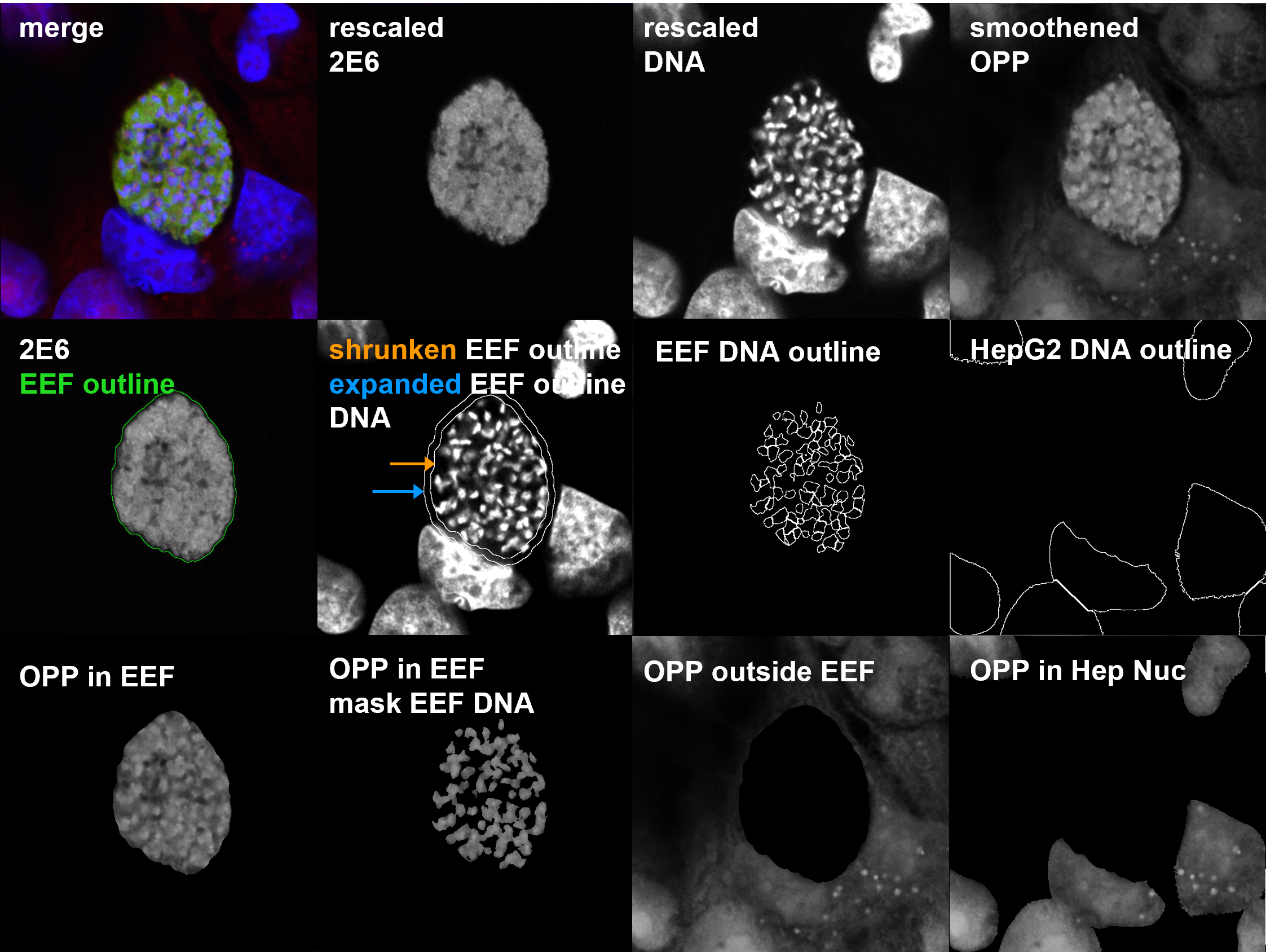
Figure 2. Tiled image example generated in CellProfiler. Tiled images provide a visual overview of the raw images, objects identified, and masking. They can be very helpful in understanding how to optimize batch segmentation parameters for a given dataset. Each tiled image is metadata-linked to the corresponding data, and image tiles for data points of interest in quality control or exploratory data analysis are routinely inspected via an interactive KNIME workflow ( https://hub.knime.com/-/spaces/-/~TZCrKvv3sbJwM_xP/current-state/). The representative parasite in this tiled image is from a 48 hours post-infection (hpi) timepoint. The shrunken exoerythrocytic form (EEF) outline indicated by the orange arrow is inside of the expanded EEF outline indicated by the blue arrow. OPP, o-propargyl puromycin.Use the MaskImage module to apply an inverse shrunken EEF object mask to both DNA and OPP-A555 images for analysis of parasite-specific fluorescence.
Critical: You need to create a unique and unambiguous name for every object and masked image generated in the CellProfiler modules, as these objects and masked images are used for downstream measurements of object area and image intensity.
In another MaskImage module, use the expanded EEF object to mask the DNA and OPP-A555 images for analysis of HepG2 features.
Apply IdentifyPrimaryObjects modules to the masked images to further define any other features of interest, such as EEF DNA objects and HepG2 DNA objects.
Using a “Tile” module, construct a tiled image (Figure 2) containing raw images, merged channels, outlines of objects from key segmentation steps, masked images, etc. Then, with the SaveImages module, define folder location where the tiles will be written and define the tiled image output name using the metadata-encoded input file names. Tiled images (Figure 2) provide a single point of reference for quality control (QC) and ground truth determination of the image contents, which we routinely examine using an interactive KNIME workflow (described in section H); an example workflow is available to download on the KNIME hub ( https://hub.knime.com/-/spaces/-/~TZCrKvv3sbJwM_xP/current-state/ ).
Use MeasureObjectSizeShape, MeasureImageAreaOccupied, and MeasureImageIntensity modules to extract features for objects and masked images that were defined in upstream modules.
Finally, use ExportToSpreadsheet module to define the output file location, naming scheme, and which features are to be exported to spreadsheets.
Note: All measurements pertaining to objects will be written into separate CSVs and the image measurements will be written to the image CSV.
Critical: If you are manually selecting which feature measurements to include, be sure to include all necessary metadata to join object features to the image CSV during data analysis steps in section H.
When the pipeline is ready to run, save a copy to disk and click Analyze images.
Data analysis
Note: We use KNIME for all data cleaning and exploratory analyses. Our ACFM workflow generates images of anything identified as meeting the fluorescence and size properties that define EEF object in the low resolution, low magnification images, but not every image from which data is extracted will meet our criteria for inclusion in downstream data analyses. To do so, the image must contain a single, centered, well-focused parasite in the HepG2 monolayer. Since we strive to meaningfully quantify single parasite variation in protein synthesis, we have iteratively optimized our QC filters (Figure 3) to meet our objective. Some images will fail QC based on the ground truth of what the image contains, while others will be filtered when segmentation failures are identified. In our analyses, each row contains data from a single ACFM image. Each image is thus passed through QC filters via the extracted data, and the entire row will be tagged and removed from the main dataset by the first filter where a QC criterion is not met. When all data have been analyzed, the filtered images then comprise a separate dataset, which is explored via an interactive dashboard to identify any systematic issues and ensure data integrity. (See the Validation section for link to our QC and exploratory data analysis workflow on the KNIME hub.) Once we have our final dataset comprised of all images that passed QC, we also perform exploratory analyses and visualizations in KNIME and prepare data for any statistical tests or visualizations in other platforms.
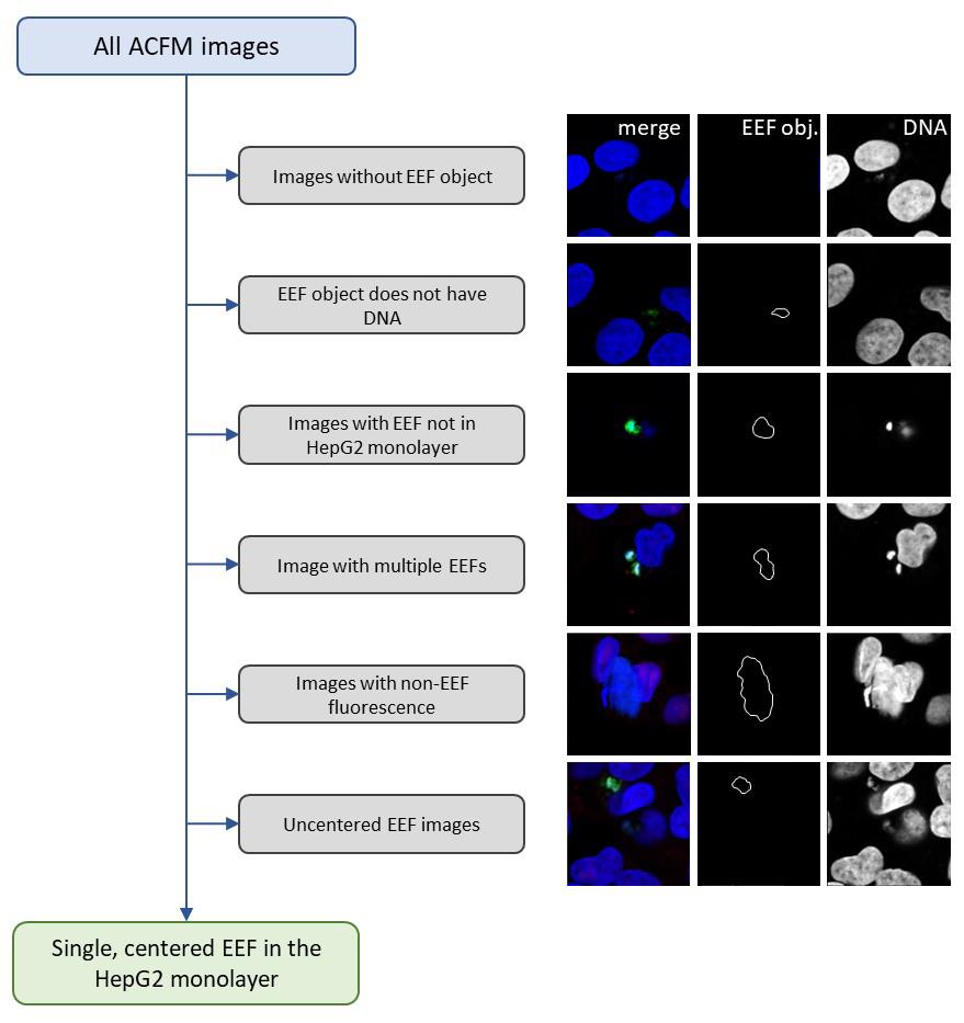
Figure 3. Image data quality control steps with example images. Quality control filters designed to identify and remove confounding image data are consistently applied across the entire dataset prior to data normalization or analysis. Example images are representative of image artifacts and image segmentation artifacts from a 28 hours post-infection (hpi) dataset. Several types of artifacts would be recognized and removed by more than one filter. ACFM, automated confocal feedback microscopy; EEF, exoerythrocytic form.
The key features extracted in CellProfiler are the fluorescence intensity values of OPP-A555 (corresponding to the 30 min nascent proteome) in both the parasite and the in-image HepG2 cells. In our 96-well plate, we have four wells of DMSO controls. Calculate the OPP-A555 mean fluorescence intensity (MFI) of all DMSO-treated EEFs parasites from the four wells. This value is set to 100.
Similarly calculate the OPP-A555 mean fluorescence intensity (MFI) of all DMSO-treated in-image HepG2 from the four wells. This value is also set to 100.
Normalize the data for each EEF and an in-image HepG2 as a percentage of the relevant DMSO control OPP MFI; e.g., if the control OPP MFI is 0.27, which is set to 100, then a well with an OPP MFI of 0.11 would be normalized to [(0.11/0.27) × 100] = 40.7
Note: In KNIME, we normalize data using the Normalize Plates (POC) node.
Use the normalized data to compare, for instance, the ability of the anisomycin control to inhibit both P. berghei liver stage and HepG2 translation in three independent experiments.
For analyses or visualizations outside of KNIME, use a CSV writer node to write datasets to disk.
Validation of protocol
This protocol has been used and validated in the following research articles:
McLellan et al., 2023. Single-cell quantitative bioimaging of Plasmodium berghei liver stage translation. mSphere. DOI: https://doi.org/10.1128/msphere.00544-23 (entire paper).
McLellan & Hanson, 2023. Translation inhibition efficacy does not determine the Plasmodium berghei liver stage antiplasmodial efficacy of protein synthesis inhibitors. BioRxiv. DOI: https://doi.org/10.1101/2023.12.07.570699 (Figures 1–3, 6C, S1–4, S6)
KNIME exploratory data analysis and QC workflows:
KNIME hub QC and exploratory data analysis interactive workflow corresponding to Figure 1 of [11]: https://hub.knime.com/-/spaces/-/~TZCrKvv3sbJwM_xP/most-recent/
KNIME hub exploratory data analysis interactive workflow with data used to generate Figure 2–3 and associated supplementary figures of [11]: https://hub.knime.com/-/spaces/-/~EcnvMwYtqylu2reV/current-state/
General notes and troubleshooting
General notes
The preferred methods for dissecting infected mosquitos and isolating sporozoites from the salivary glands tend to vary from laboratory to laboratory, and detailed protocols for several of these approaches have been previously published.
Mosquito dissection:
A detailed Bio-protocol from the Kyle group [18] outlines the isolation of salivary glands from Anopheles dirus in section E, steps 1–8. This also includes a video demonstrating the dissection steps in video 2.
Another Bio-protocol [19] provides a step-by-step tutorial on salivary gland removal from non-infected mosquitos with detailed diagrams.
For detailed videos of mosquito dissection and salivary gland removal, please see the Journal of Visual Experiments [20] and the Wellcome Trust film unit [21]. These contain accurate depictions of what isolated salivary glands look like under a dissection microscope.
Sporozoite isolation from salivary glands:
A protocol for sporozoite isolation and counting from the Sinnis laboratory website [22] details their use of a Dounce homogenizer to disrupt the salivary glands and isolate the sporozoites by centrifugation.
Another previous Bio-protocol [23] outlines their use of a Teflon homogenizer and filtering steps to isolate sporozoites.
A protocol for the dissection-independent isolation of sporozoites from whole-mosquito lysates using a gradient centrifugation [24] highlights an alternative approach.
Example images of sporozoites visualized with transmitted light microscopy are available in Figure 5A of [25] and Figure 1A [26].
While we detail a 4 h compound pretreatment format here, the OPP assay is very flexible. We have also extensively run the assay in competition (co-OPP) mode, where a compound of interest is added at the same time as OPP. Known direct translation inhibitors show similar potency and efficacy in co-OPP and acute pretreatment assays [10], and we would recommend co-OPP mode to test whether an uncharacterized compound of interest likely functions as a Plasmodium translation inhibitor. We have used a 30 min period of OPP labeling without compound treatment to visualize translation throughout P. berghei liver-stage development, from sporozoites to hepatic merozoites. As parasite size and shape change dramatically during development, parameters for image acquisition, segmentation, feature extraction, and QC will need to be adjusted accordingly for quantification. We have also demonstrated specific OPP-A555 labeling in P. falciparum blood-stage parasites, from ring stages to schizonts, and others have used OPP labeling to quantify P. falciparum asexual blood-stage translation using flow cytometry [27]. We only use a 30 min period of OPP labeling for quantifying P. berghei translation, but we have been able to visualize the P. berghei nascent proteome with OPP treatments periods as short as 5 min.
In addition to the 96-well plate format described in the main protocol, we also quantify translation indirectly infecting HepG2 monolayers cultured on glass coverslips in a 24-well plate. The protocol is identical with the following exceptions:
Section B, Step 1: 75,000 HepG2 cells are seeded in 500 µL per well onto a glass coverslip. After dispensing cell seeding suspension to each well, use the pipette tip to gently press the coverslip to the bottom of the dish to avoid cells attaching to the bottom of the coverslip.
Section C, Step 10: Coverslips are infected with a maximum of 50,000 sporozoites/well, but the minimum number can be adjusted depending on imaging modality and sporozoite availability.
Section C, Step 14: Instead of detaching and reseeding infected cells, remove the plate from the incubator, aspirate the sporozoite suspension media, and replace with 1 mL of fresh iDMEM. Then, return to incubator and move on to step D.
Section D, several steps: The volumes during treatment and OPP labeling are increased to account for larger well volumes. Compound pretreatments are performed using 500 µL for each well and OPP labeling is performed in 300 µL.
Section E, several steps: Use 500 µL for permeabilization and wash steps. To perform a click reaction on a coverslip (CS), remove the CS from 2% BBS using coverslip forceps, gently blot the edge on a paper towel to wick away BBS solution, place inverted CS on a piece of parafilm (cells facing up), and dispense 30 µL of click reaction MM. We have found that using a tinfoil-covered slide-box containing a water-saturated Kimwipe works well to prevent evaporation of the MM during the click reaction. Return the CS to the 24-well plate for PBS washes. Antibody labeling steps are performed in the same way. After labeling is completed, mount coverslips onto a glass slide, cell side down, into a drop of Fluoromount-G and allow them to cure overnight before imaging.
HepG2 cells are available from ATCC (item number HB-8065) and other national cell banks. If you source HepG2 cells from ATCC or start from any HepG2 cell stock in which the cells grow largely in clumps, you will likely need to perform several cell passages in a 12.5 cm2 dish/flask (or smaller, if necessary), removing the clumped cells as described in Procedure section A, until enough cells are recovered to scale up the culture.
Troubleshooting
Problem 1: Low iHepG recovery during trypsinization.
Possible cause: Failure to dislodge all cells from the plastic.
Solution: As noted in section C steps 17–18, add 200 µL of iDMEM to each well immediately after collecting the cell suspension and carefully inspect each well on a phase contrast microscope to make sure that no cells remain attached to the substrate. This can be done multiple times if necessary. iHepG2 (exposed to sporozoite solution) are noticeably more difficult to detach from the plastic substrate than uninfected HepG2.
Acknowledgments
The iHepG2 recovery and reseeding protocol was first developed for work supported by the Bill and Melinda Gates Foundation (OPP1141284 to KKH). P. berghei liver-stage protein synthesis quantification assay development was supported by the National Institutes of Health (R21AI149275 to KKH). JLM was supported by a South Texas Center for Emerging Infectious Diseases fellowship. The protocol was adapted from the publication McLellan et al. [10] and preprint McLellan and Hanson [11].
Competing interests
The authors declare no competing interests.
References
- Prudêncio, M., Rodriguez, A. and Mota, M. M. (2006). The silent path to thousands of merozoites: the Plasmodium liver stage. Nat. Rev. Microbiol. 4(11): 849–856. https://doi.org/10.1038/nrmicro1529.
- Calvocalle, J. M., Moreno, A., Eling, W. M. C. and Nardin, E. H. (1994). In Vitro Development of Infectious Liver Stages of P. yoelii and P. berghei Malaria in Human Cell Lines. Exp. Parasitol. 79(3): 362–373. https://doi.org/10.1006/expr.1994.1098.
- Hollingdale, M. R., Leland, P., Leef, J. L. and Beaudoin, R. L. (1983). The Influence of Cell Type and Culture Medium on the In vitro Cultivation of Exoerythrocytic Stages of Plasmodium berghei. J. Parasitol. 69(2): 346–352. https://doi.org/10.2307/3281232.
- Gissen, P. and Arias, I. M. (2015). Structural and functional hepatocyte polarity and liver disease. J. Hepatol. 63(4): 1023–1037. https://doi.org/https://doi.org/10.1016/j.jhep.2015.06.015.
- Treyer, A. and Müsch, A. (2013). Hepatocyte polarity. Compr. Physiol. 3(1): 243–287. https://doi.org/10.1002/cphy.c120009.
- Hoehme, S., Brulport, M., Bauer, A., Bedawy, E., Schormann, W., Hermes, M., Puppe, V., Gebhardt, R., Zellmer, S., Schwarz, M., et al. (2010). Prediction and validation of cell alignment along microvessels as order principle to restore tissue architecture in liver regeneration. Proc. Natl. Acad. Sci. U.S.A. 107(23): 10371–10376. https://doi.org/doi:10.1073/pnas.0909374107.
- Ahyong, V., Sheridan, C. M., Leon, K. E., Witchley, J. N., Diep, J. and DeRisi, J. L. (2016). Identification of Plasmodium falciparum specific translation inhibitors from the MMV Malaria Box using a high throughput in vitro translation screen. Malar. J. 15: 173. https://doi.org/10.1186/s12936-016-1231-8.
- Sheridan, C. M., Garcia, V. E., Ahyong, V. and DeRisi, J. L. (2018). The Plasmodium falciparum cytoplasmic translation apparatus: a promising therapeutic target not yet exploited by clinically approved anti-malarials. Malar. J. 17(1): 465. https://doi.org/10.1186/s12936-018-2616-7.
- Tamaki, F., Fisher, F., Milne, R., Terán, F. S.-R., Wiedemar, N., Wrobel, K., Edwards, D., Baumann, H., Gilbert, I. H., Baragana, B., et al. (2022). High-Throughput Screening Platform To Identify Inhibitors of Protein Synthesis with Potential for the Treatment of Malaria. Antimicrob. Agents. Chemother. 66(6): e00237–00222. https://doi.org/doi:10.1128/aac.00237-22.
- McLellan, J. L., Sausman, W., Reers, A. B., Bunnik, E. M. and Hanson, K. K. (2023). Single-cell quantitative bioimaging of P. berghei liver stage translation. mSphere 0(0): e0054423. https://doi.org/10.1128/msphere.00544-23.
- McLellan, J. L. and Hanson, K. K. (2023). Translation inhibition efficacy does not determine the Plasmodium berghei liver stage antiplasmodial efficacy of protein synthesis inhibitors. bioRxiv: 2023.2012.2007.570699. https://doi.org/10.1101/2023.12.07.570699.
- Liu, J., Xu, Y., Stoleru, D. and Salic, A. (2012). Imaging protein synthesis in cells and tissues with an alkyne analog of puromycin. Proc. Natl. Acad. Sci. U.S.A. 109(2): 413–418. https://doi.org/10.1073/pnas.1111561108.
- Tsuji, M., Mattei, D., Nussenzweig, R. S., Eichinger, D. and Zavala, F. (1994). Demonstration of heat-shock protein 70 in the sporozoite stage of malaria parasites. Parasitol. Res. 80(1): 16–21. https://doi.org/10.1007/BF00932618.
- Hilsenstein, V. (2017). LCC Modules for CellProfiler. (Accessed on Jan 22, 2024, https://github.com/VolkerH/MatrixScreenerCellprofiler/wiki)
- Tischer, C., Hilsenstein, V., Hanson, K. and Pepperkok, R. (2014). Adaptive fluorescence microscopy by online feedback image analysis. Methods Cell Biol. 123: 489–503. https://doi.org/10.1016/B978-0-12-420138-5.00026-4.
- Sarkans, U., Chiu, W., Collinson, L., Darrow, M. C., Ellenberg, J., Grunwald, D., Hériché, J.-K., Iudin, A., Martins, G. G., Meehan, T., et al. (2021). REMBI: Recommended Metadata for Biological Images—enabling reuse of microscopy data in biology. Nat. Methods 18(12): 1418–1422. https://doi.org/10.1038/s41592-021-01166-8.
- Senft, R. A., Diaz-Rohrer, B., Colarusso, P., Swift, L., Jamali, N., Jambor, H., Pengo, T., Brideau, C., Llopis, P. M., Uhlmann, V., et al. (2023). A biologist’s guide to planning and performing quantitative bioimaging experiments. PLoS Biology 21(6): e3002167. https://doi.org/10.1371/journal.pbio.3002167.
- Maher, S. P., Vantaux, A., Cooper, C. A., Chasen, N. M., Cheng, W. T., Joyner, C. J., Manetsch, R., Witkowski, B. and Kyle, D. (2021). A Phenotypic Screen for the Liver Stages of Plasmodium vivax. Bio Protoc. 11(23): e4253. https://doi.org/10.21769/BioProtoc.4253.
- Schmid, M. A., Kauffman, E., Payne, A., Harris, E. and Kramer, L. D. (2017). Preparation of Mosquito Salivary Gland Extract and Intradermal Inoculation of Mice. Bio Protoc. 7(14). https://doi.org/10.21769/BioProtoc.2407.
- Coleman, J., Juhn, J. and James, A. A. (2007). Dissection of midgut and salivary glands from Ae. aegypti mosquitoes. J. Vis. Exp. (5): 228. https://doi.org/10.3791/228.
- Collection, W. (1953). The dissection of a mosquito for malaria parasite. Wellcome Trust 1953; 2008. (Accessed on Jan 16, 2024, https://wellcomecollection.org/works/wrxrzyv7)
- Coppi, A. and Sinnis, P. (Accessed Jan 16, 2024). Isolation of Plasmodium Sporozoites from Mosquito Salivary Glands. (Accessed on Jan 16, 2024, https://sinnislab.johnshopkins.edu/#protocols)
- Gupta, D. K. and Diagana, T. (2020). In vitro Cultivation and Visualization of Malaria Liver Stages in Primary Simian Hepatocytes. Bio Protoc. 10(16): e3722. https://doi.org/10.21769/BioProtoc.3722.
- Blight, J., Sala, K. A., Atcheson, E., Kramer, H., El-Turabi, A., Real, E., Dahalan, F. A., Bettencourt, P., Dickinson-Craig, E., Alves, E., et al. (2021). Dissection-independent production of Plasmodium sporozoites from whole mosquitoes. Life Sci. Alliance 4(7): e202101094. https://doi.org/10.26508/lsa.202101094.
- Montagna, G. N., Buscaglia, C. A., Münter, S., Goosmann, C., Frischknecht, F., Brinkmann, V. and Matuschewski, K. (2012). Critical Role for Heat Shock Protein 20 (HSP20) in Migration of Malarial Sporozoites. J. Biol. Chem. 287(4): 2410–2422. https://doi.org/10.1074/jbc.M111.302109.
- Battista, A., Frischknecht, F. and Schwarz, U. S. (2014). Geometrical model for malaria parasite migration in structured environments. Phy. Rev. E 90(4): 042720. https://doi.org/10.1103/PhysRevE.90.042720.
- Xie, S. C., Metcalfe, R. D., Dunn, E., Morton, C. J., Huang, S. C., Puhalovich, T., Du, Y., Wittlin, S., Nie, S., Luth, M. R., et al. (2022). Reaction hijacking of tyrosine tRNA synthetase as a new whole-of-life-cycle antimalarial strategy. Science 376(6597): 1074–1079. https://doi.org/10.1126/science.abn0611.
Article Information
Copyright
© 2024 The Author(s); This is an open access article under the CC BY-NC license (https://creativecommons.org/licenses/by-nc/4.0/).
How to cite
McLellan, J. L., Garcia-Vilanova, A. and Hanson, K. K. (2024). An Optimized P. berghei Liver Stage–HepG2 Infection Model for Simultaneous Quantitative Bioimaging of Host and Parasite Nascent Proteomes. Bio-protocol 14(5): e4952. DOI: 10.21769/BioProtoc.4952.
Category
Microbiology > Microbial cell biology > Cell-based analysis
Cell Biology > Cell imaging > Fluorescence
Do you have any questions about this protocol?
Post your question to gather feedback from the community. We will also invite the authors of this article to respond.