- Protocols

- Articles and Issues
- For Authors
- About
- Become a Reviewer

A Versatile Pipeline for High-fidelity Imaging and Analysis of Vascular Networks Across the Body
Published: Vol 14, Iss 4, Feb 20, 2024 DOI: 10.21769/BioProtoc.4938 Views: 3044
Reviewed by: Pilar Villacampa AlcubierreXiaokang Wu
Original research article
The authors used this protocol in:
Jul 2022
Advertisement


Protocol Collections
Comprehensive collections of detailed, peer-reviewed protocols focusing on specific topics


Abstract
Structural and functional changes in vascular networks play a vital role during development, causing or contributing to the pathophysiology of injury and disease. Current methods to trace and image the vasculature in laboratory settings have proven inconsistent, inaccurate, and labor intensive, lacking the inherent three-dimensional structure of vasculature. Here, we provide a robust and highly reproducible method to image and quantify changes in vascular networks down to the capillary level. The method combines vasculature tracing, tissue clearing, and three-dimensional imaging techniques with vessel segmentation using AI-based convolutional reconstruction to rapidly process large, unsectioned tissue specimens throughout the body with high fidelity. The practicality and scalability of our protocol offer application across various fields of biomedical sciences. Obviating the need for sectioning of samples, this method will expedite qualitative and quantitative analyses of vascular networks. Preparation of the fluorescent gel perfusate takes < 30 min per study. Transcardiac perfusion and vasculature tracing takes approximately 20 min, while dissection of tissue samples ranges from 5 to 15 min depending on the tissue of interest. The tissue clearing protocol takes approximately 24–48 h per whole-tissue sample. Lastly, three-dimensional imaging and analysis can be completed in one day. The entire procedure can be carried out by a competent graduate student or experienced technician.
Key features
• This robust and highly reproducible method allows users to image and quantify changes in vascular networks down to the capillary level.
• Three-dimensional imaging techniques with vessel segmentation enable rapid processing of large, unsectioned tissue specimens throughout the body.
• It takes approximately 2–3 days for sample preparation, three-dimensional imaging, and analysis.
• The user-friendly pipeline can be completed by experienced and non-experienced users.
Graphical overview
Background
Vasculature plays a key role during the growth, maintenance, and repair of tissues throughout the body. Accumulating evidence suggests that the slow and protracted reorganization of vascular networks can promote recovery of function (Felmeden et al., 2003; Evans et al., 2021) but may also contribute to neuropathological hallmarks of injury and disease (Ostergaard et al., 2016).
A critical point to consider is that standard methods to study vasculature changes in laboratory settings have proven inaccurate and labor-intensive, lacking the inherent three-dimensional structure of the vasculature. Conventionally, visualization of blood vessels in tissues of interest often employs immunohistochemical (IHC) techniques. This approach uses thin tissue sections to detect endothelial cells through vessel wall stains. The resulting two-dimensional images do not capture the inherent three-dimensional, tortuous structure of vasculature networks (Rust et al., 2020). Furthermore, IHC is a multistep process, increasing the likelihood of introducing error, non-experimental variables (e.g., lot-to-lot variability that contributes to inconsistent results in assays using antibodies), or experimenter bias to analysis, as only a small fraction of the tissue is typically processed. Thus, quantifying the vascular response to injury or disease is often limited to the mean fluorescent intensity of IHC stains, which is highly dependent on technical consistency and subject to bias (Marien et al., 2016; Cheung et al., 2020). Methods of three-dimensional imaging of vasculature networks are currently available. However, they are niche in their applications throughout the body and are largely constrained by expensive or otherwise inaccessible imaging equipment and methodologies including tomography, magnetic resonance imaging, and photoacoustic imaging (Xiong et al., 2017; Pac et al., 2022; Menozzi et al., 2023).
To overcome these barriers, we have developed a practical and accessible pipeline that permits robust and highly reproducible qualitative and quantitative three-dimensional analysis of vascular networks that can resolve changes to the capillary level. Initially, we detail our approach for vasculature tracing and preparing unsectioned tissue samples throughout the body. Then, we present a methodology for optically clearing neuronal and non-neuronal tissues (Susaki et al., 2015) and provide the necessary steps to acquire three-dimensional images using conventional laser scanning confocal microscopy. Lastly, we detail our pipeline for vessel segmentation using AI-based convolutional reconstruction (Imaris software, paid subscription) or semi-automated three-dimensional reconstruction (ImageJ software, freely available). This framework can consistently capture subtle changes in capillary structure such as total length, branching points, branch length, and diameter of vessels, providing a robust and user-friendly approach to study vascular networks in health and disease. Additionally, this scalable method can be adapted for volumetric imaging and analysis of vasculature structures in a variety of preclinical models, thus accelerating translation of promising findings to large animals and non-human primates.
Materials and reagents
Biological materials
Adult (7–8-week-old) female and male C57BL/6J mice (The Jackson Laboratory, stock number: 000664)
Reagents
Paraformaldehyde (PFA) (Sigma, catalog number: 441244)
Ketamine hydrochloride (100 mg/mL) (Covertrus, catalog number: 071069)
Xylazine hydrochloride (100 mg/mL) (Rompun)
Albumin-tetramethylrhodamine isothiocyanate bovine (albumin-TRITC) (Sigma, catalog number: A2289)
0.9% Isotonic saline solution (B. Braun, catalog number: R5200)
Gelatin from porcine skin (Sigma, catalog number: G1890)
Phosphate buffered saline (PBS) (Gibco, catalog number: 21600-044)
Urea (Bio-Rad, catalog number: 161-0731)
Quadrol [N,N,N’,N’-Tetrakis(2-hydroxypropyl)ethylenediamine] (Sigma, catalog number: 122262)
Triton-X 100 (Sigma, catalog number: T9284)
Solutions
4% PFA (see Recipes)
80 wt% Quadrol (see Recipes)
Clearing solution (see Recipes)
Gel perfusate (see Recipes)
Ketamine/Xylazine mixture (see Recipes)
Recipes
4% PFA
Reagent Final Concentration Quantity PFA 4% 40 g PBS 1× 1,000 mL Total 4% 1,000 mL 80 wt% Quadrol
Reagent Final Concentration Quantity Quadrol 80 wt% 500 g dH2O n/a 125 g Total 80 wt% 625 g Clearing solution
Reagent Final Concentration Quantity 80 wt% Quadrol 80% 156 g Urea n/a 125 g dH2O n/a 144 g Triton-X 100 n/a 75 g Total 80% 500 g Gel perfusate
Reagent Final Concentration Quantity Gelatin from porcine skin 2% 0.1 g/5 mL Albumin-TRITC 0.05% 2.5 mg/5 mL PBS 1× 5 mL/mouse Total n/a n/a Ketamine/Xylazine anesthetic
Reagent Final Concentration Quantity Ketamine 150 mg/kg body weight n/a Xylazine hydrochloride 15 mg/kg body weight n/a Final n/a
Laboratory supplies
Aluminum foil (Fisher Scientific, Fisherbrand, catalog number: 01-213-100)
Microruler (Fine Science Tools, catalog number: 30086-30)
Fluted filter paper circles (Fisher Scientific, Fisherbrand, catalog number: 09-790-14D)
2 mL Eppendorf tube (Eppendorf, catalog number: 022363352)
50 mL conical centrifuge tube (VWR, catalog number: 89039-656)
100 mL glass beaker (Pyrex, Corning, catalog number: 1000-100)
Glass coverslip (Fisher Scientific, catalog number: 1254588)
Microscope glass slides (Fisher Scientific, Fisherbrand, catalog number: 12-550-15)
23 G needle (BD Biosciences, catalog number: 305193)
10 mL syringe (Henry Schein, catalog number: 570-2620)
1 L round media storage bottle (Pyrex, catalog number: GL45)
Equipment
Vacuum desiccator (Thermo Scientific, catalog number: 08-642-5)
Peristaltic pump (Cole-Parmer, Masterflex, catalog number: 07525)
Vortex mixer (VWR, catalog number: BV1000-GM)
Hotplate stirrer (Benchmark Scientific, catalog number: H400-HS)
Laser scanning microscope (Nikon, model: C2 plus)
Dissection microscope (Zeiss, model: Stemi 2000, catalog number: SP-STEMI2000-TS2)
Computer with 3.3 GHz CPU (Intel or AMD) 6–8 cores, 32–64 GB of RAM, NVIDA Quadro RTX 4000 (8 GB), and multiple fast hard disks or (SATA) SSDs (recommended system when using Imaris software)
Software and datasets
Imaris Microscopy Image Analysis software (Bitplane, Oxford Instruments, v10.0, RRID: SCR_007370) https://imaris.oxinst.com/products/imaris-for-neuroscientists
Free alternative software: FIJI/ImageJ (NIH, RRID: SCR_002285) https://imagej.nih.gov/ij/download.html)
Excel (Microsoft, https://www.microsoft.com/en-us/microsoft-365/p/excel/cfq7ttc0hr4r?activetab=pivot:overviewtab)
Procedure
4% PFA preparation
In a chemical fume hood, heat 600 mL of PBS to 65 °C while stirring on a hotplate stirrer.
Add 40 g of PFA and continue stirring for approximately 5 min.
While stirring, turn down the heat and add 1 M NaOH dropwise until the solution is clear.
Cool the solution immediately on ice for approximately 30 min.
Buffer the solution with 1 M HCl as needed to obtain a pH of 7.4.
Add PBS to 1 L; then, filter using a fluted filter paper into a 1 L glass bottle.
Store at 4 °C until ready to use.
Clearing solution preparation
Note: Liquids are measured by volume as well as weight. Quadrol is a highly viscous liquid; therefore, an 80 wt% working solution is used.
Prepare 80 wt% Quadrol:
Add 125 g of dH2O to 500 g of Quadrol. We suggest measuring liquids by weight during the preparation of the clearing solution.
Stir for at least 30 min. This solution can be stored at room temperature for approximately six months.
Mix 125 g of urea with 156 g of 80 wt% Quadrol in 144 g of dH2O.
Use a heated stirrer at low–medium temperature.
Once the solution is homogenous and fully dissolved, remove it from heat and continue stirring at room temperature.
Add 75 g of Triton X-100 and continue stirring for ~1 min.
Degas the solution using a vacuum desiccator at ~0.1 MPa for ~30 min or until bubbles are removed from the solution.
Store at room temperature and protected from light for up to six months.
Gel perfusate preparation
Note: The following procedure will require a minimum of 5 mL of PBS per mouse. When determining the amount of gelatin to make, it is best to factor in approximately 10%–20% to compensate for repetitive injections.
Calculate the necessary quantity of sterile PBS, gelatin powder, and albumin-TRITC conjugate for samples.
The concentration of gelatin is 2% in PBS while albumin-TRITC concentration is 0.05% of the gelatin mixture volume.
Store the measured albumin-TRITC in a 2 mL Eppendorf tube in a 4 °C refrigerator until adding it to the solution in step 7.
Wrap the tube in aluminum foil to protect the compound from light.
Prepare the 2% gelatin mixture.
Transfer PBS to a glass beaker and begin heating until simmering or lightly boiling. Cover the beaker to prevent liquid loss while heating.
Add a small stir bar and begin gradually adding the gelatin powder while stirring.
Reduce heat to a simmer and continue stirring for ~5 min or until the powder is completely dissolved.
Transfer the gelatin mixture to a 50 mL conical tube and allow the temperature to stabilize at 45 °C in the heated water bath.
Remove 1 mL of gelatin mixture from the conical tube, add it to the 2 mL Eppendorf tube containing the albumin-TRITC from step 2, mix the solution using a vortex mixer, and transfer the mixture back to the 50 mL conical tube.
Place the 50 mL conical tube in a 45 °C heated water bath.
Perfusion and vessel labeling
Weigh the mice and administer the ketamine (150 mg/kg body weight) and xylazine (15 mg/kg body weight) mixture (see Recipes) intraperitoneally. Determine if the animal is deeply anesthetized using the toe pinch reflex.
Prepare 30 mL of 1× PBS per adult mouse and 100 mL of 4% PFA in PBS (see Recipes) for perfusion, pour into glass beakers, and connect to pump (Figure 1A). Prefill tubing with 1× PBS and remove any air bubbles.
Position the mouse on a dissection board and secure limbs using small pins (Figure 1A). Locate the edge of the rib cage and make a small incision into the abdominal cavity. Without damaging the heart, open the thoracic cavity by cutting along either side of the rib cage.
Insert the 23 G needle connected to 1× PBS into the left ventricle (Figures 1B and 1C), make a small cut into the right atrium, and begin perfusion for 3 min at a rate of 10 mL/min to clear the vasculature of blood and red blood cells.
Critical: Be careful not to puncture the septum as this will result in poor/no perfusion and vasculature labeling. Also, be sure to cut the right atrium before turning on the pump to prevent capillary collapse or damage.
After flushing with PBS, pause the peristaltic pump and transfer the tubing to ice-cold 4% PFA. Resume perfusion for 10 min at a rate of 10 mL/min. The pausing prevents air bubbles from entering the tube. If performed correctly, the body will harden a few minutes after injecting the fixative (4% PFA).
Figure 1. Mouse perfusion and injection of the gel perfusate. (A) Representative images of the perfusion setup and a deeply anesthetized adult mouse fixed on a dissection board. (B) Schematic of mouse heart. The syringe needle is inserted into the left ventricle (arrow). After making a small cut into the right atrium, the peristaltic pump is turned on and mouse perfusion begins. (C) Representative images of how to insert the syringe needle into the left ventricle of an adult mouse. Right panel: higher magnification of the region indicated by the dashed line. (D) Representative image of how to insert the syringe needle during the injection of the gel perfusate.When approaching 8–9 min, remove the fluorescent gel perfusate from the heated water bath.
Draw up 5 mL into a 10 mL syringe and place the fluorescent gel perfusate back into the water bath.
After 10 min, stop the pump and quickly remove the needle from the heart. Using a 23 G needle, slowly inject 5 mL of the fluorescent gel perfusate into the left ventricle (use the same opening as before) over 30 s to match the rate of fixative perfusion (Figure 1D).
Clamp the right atrium with a hemostat immediately after finishing.
Remove the mouse from the dissection board and place it on ice for 30 min to allow gel polymerization.
Note: Place a plastic or hydrophobic covering over the ice so that the mouse does not get wet.
Carefully remove the hemostat clamp and prepare for dissection.
Note: It may be useful to post-fix the animal(s) in approximately 50 mL of 4% PFA at 4 °C overnight, depending on the tissue of interest and quality of fixation.
Tissue isolation and optical clearing
Begin dissection of the necessary tissue.
Predetermine regions of interest before clearing tissue. Remove any debris that may obscure the view during image acquisition, as it will be difficult to see following tissue clearing.
Note: The samples can be kept in 1× PBS at 4 °C until they need to be cleared. Once the samples have been cleared, do not immerse them in another liquid. This will alter the refractive index within the tissue and impede optimal imaging.
Place the samples in the appropriate volume of clearing solution (see Recipes) and incubate according to Table 1 at 37 °C.
Table 1. Tissue clearing (neuronal and non-neuronal tissues originating from adult mice)
Tissue Incubation time Solution volume Brain 7 days 3.0 mL Spinal cord 24 h 1.0 mL Dorsal root ganglion 24 h 0.5 mL Optic nerve and chiasm 24 h 0.5 mL Facial nerve 24 h 0.5 mL Sciatic nerve 24 h 0.5 mL Adrenal gland 24 h 1.0 mL Heart 48 h 1.0 mL Kidney 48 h 1.0 mL Intestines 48 h 1.0 mL Muscle 48 h 1.0 mL
Sample mounting and three-dimensional imaging
Gently remove samples from the clearing solution and place them on a microscope glass slide (Figure 2). If using a confocal microscope equipped with conventional optics with a working distance of < 4 mm, imaging of thick tissue samples (e.g., adult mouse brain) will require cutting a portion of the tissue (2–3 mm thick).
Roll two pieces of Blu-Tack into cylinders. The cylinders should be approximately 2–3 cm long and slightly thicker than the sample.
Figure 2. Tissue sample mounting for three-dimensional imaging using an upright laser scanning microscope. Representative image of a cleared mouse spinal cord mounted on a microscope glass slide and covered with a glass coverslip held in place by two pieces of modeling clay (R: rostral, C: caudal).Mount the cylinders near the edges of the glass slide, parallel to the long axis of the slide (Figure 2).
Place the tissue sample in the middle of the slide, parallel to the Blue-Tack cylinders.
Ensure the sample is properly aligned, especially if the sample requires the use of the tiling function while imaging.
Put a small drop of clearing solution (~50 µL) onto the sample. Ensure the solution does not touch the putty.
Place a glass coverslip (thickness: No. 1) on top of the sample and gently apply pressure on top of the putty.
When pressing, ensure the pressure is firm enough that a small pool forms around the sample and the coverslip is adequately held in place. Take care not to compress the sample too much, as this will distort the sample during imaging.
Position the sample under the microscope and locate the region of interest using a low magnification, long-working distance objective. If necessary, switch to a higher magnification objective (e.g., 20× with at least 1 mm working distance and high numerical aperture) and select the imaging area.
Image albumin-TRITC-filled vascular networks using an excitation wavelength of 544 nm and an emission wavelength of 570 nm (Figures 3 and 4). TRITC is a bright-orange fluorescent dye with a 557 nm maximum excitation.
Critical: Be sure to check the specification of your laser scanning microscope to determine whether the 557 nm excitation maximum is far away from your laser line. Alternatively, consider using albumin-FITC (excitation peak of 490 nm) instead of albumin-TRITC.
Figure 3. Vasculature tracing, tissue clearing, and three-dimensional imaging enable visualization of vasculature networks in neuronal tissues. (A) Representative images of whole organs and neuronal tissue samples before and after clearing. Scale bars: 2 mm. Representative fluorescence images (maximum intensity projections) of albumin-TRITC filled vasculature networks within the mouse (B) somatosensory cortex, (C) spinal cord (low thoracic-lumbar segment), (D) lumbar dorsal root ganglion (DRG), (E) facial nerve, (F) sciatic nerve, and (G) the optic nerve and chiasm. All images were acquired using a conventional laser scanning confocal microscope equipped with a long-working distance air objective (magnification: 10×; working distance: 4 mm; numerical aperture: 0.45). Scale bars: 200 µm.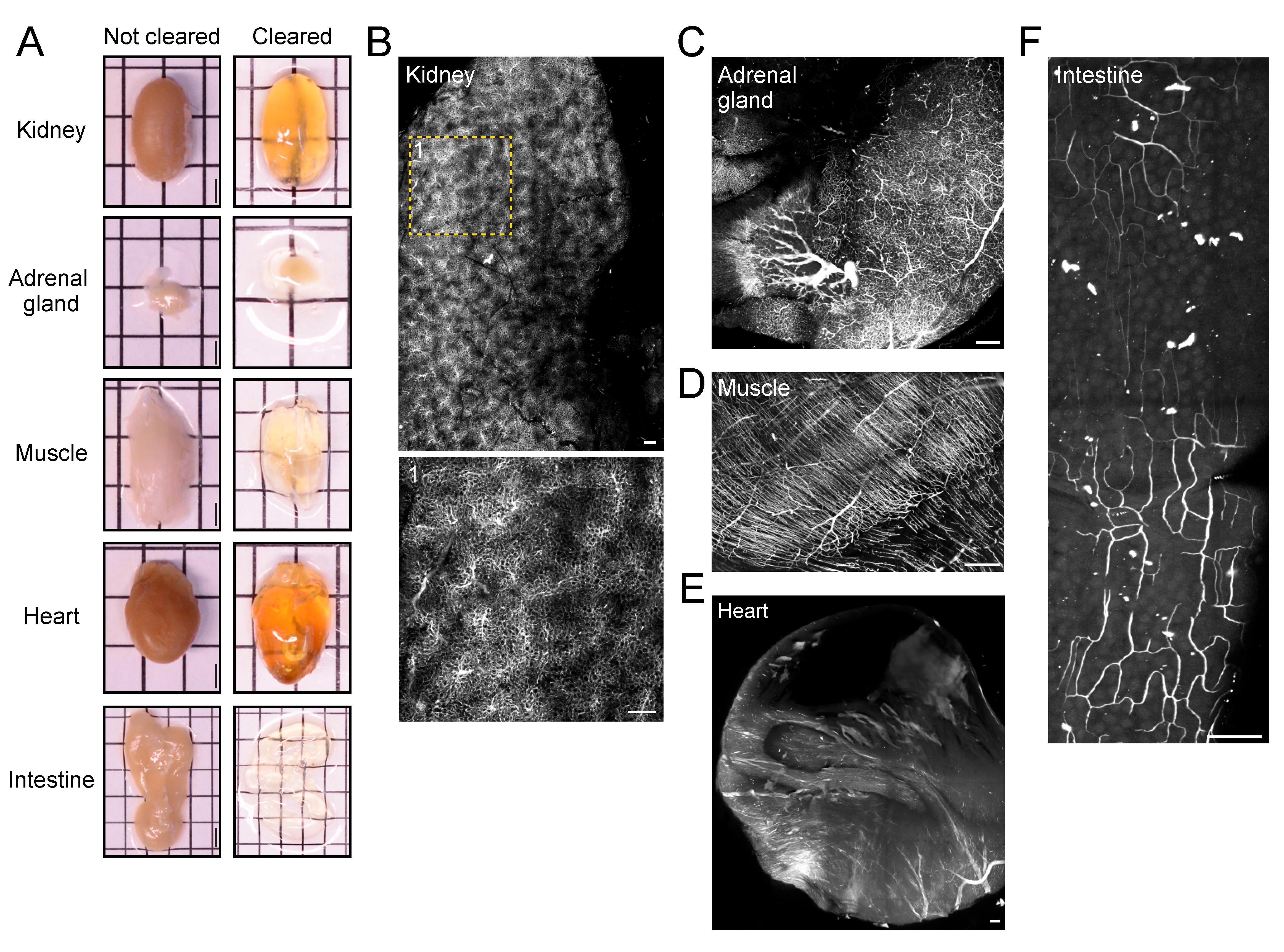
Figure 4. Vasculature tracing, tissue clearing, and three-dimensional imaging enable visualization of vasculature networks in non-neuronal tissues. (A) Before and after clearing images of whole organs and non-neuronal tissue samples. Scale bars: 2 mm. Representative fluorescence images (maximum intensity projections) of albumin-TRITC-filled vasculature networks within the mouse (B) kidney, (C) adrenal gland, (D) hindlimb muscle (gastrocnemius), (E) heart, and (F) intestine (duodenum). All images were acquired using a conventional laser-scanning confocal microscope equipped with a long-working distance air objective (magnification: 10×; working distance: 4 mm; numerical aperture: 0.45). Scale bars: 200 µm.Select the mode Frame Scan and set the image size to 1,024 × 1,024 pixels. Adjust the laser speed, laser power, and gain to obtain high-quality, high-contrast, and low-background images. If necessary, use the range indicator to adjust acquisition parameters and avoid pixel saturation. Adjust line averaging to 2 to reduce background noise.
Select the imaging depth in the z-axis (< 1.5–2 mm depending on the tissue of interest) and adjust the step size accordingly. When using a 10× objective, the z-step should be 4–5 µm.
Three-dimensional reconstruction and analysis
Open Imaris and select Surpass > File > Open to import desired file(s). Files can also be dragged and dropped into the Arena interface.
Select Arena > Observe Folder for the software to recognize folders.
Convert file to .ims by double-clicking on file(s).
Note: This is a non-destructive process that will create a copy of the original file.
Select Surpass to see a three-dimensional view of the file.
Crop the file by selecting Edit > 3D Crop.
Determine a region of interest (ROI) for your sample and drag the ROI box over that location. The dimensions can be changed by either dragging the corners of the box or typing in dimensions as described below.
Input desired dimensions in the x, y, and z planes under the drop-down boxes titled Size.
The ROI can be moved by left-clicking and dragging the box while still maintaining the specified dimensions.
Begin surface creation by clicking on the blue globular button (fourth from the left).
Open the surface wizard by clicking on the Creation/wand button (second from left) within the surface properties window (Figure 5A). No options need to be selected in the first window.
Select the vasculature channel via the Source Channel window (Figure 5A).
Select Background Subtraction and adjust the diameter of the largest sphere to the largest diameter vessel found within the image.
To measure the diameter of vessels, select the Slice button at the top of the window (to the right of 3D view).
Left-click on each side of the largest vessel to measure the distance between the two points. The measurement can be found within the docked window on the right side under Distance.
Adjust the threshold by dragging the bar within the background subtraction threshold window until the vasculature source signal is sufficiently covered by the surface. This surface represents the volume of the new mask.
Note: There will need to be a compromise between the larger and smaller vessels, as the smaller vessels can become engorged. Ensure the desired vasculature and continuous vessels are accurately represented.
Adjust filters as needed to reduce background labeling. Surfaces can be filtered according to volume, size, or other parameters by clicking on the drop-down menu.
Allow the surface to render and then mask the surface over the vasculature channel.
Select the pencil icon (fourth from left) and select Mask All....
Select the source channel for the vasculature and then click Ok. This will create a new vasculature channel only encompassing what is occupied within the surface. There will now be two channels within the Display Adjustment window.
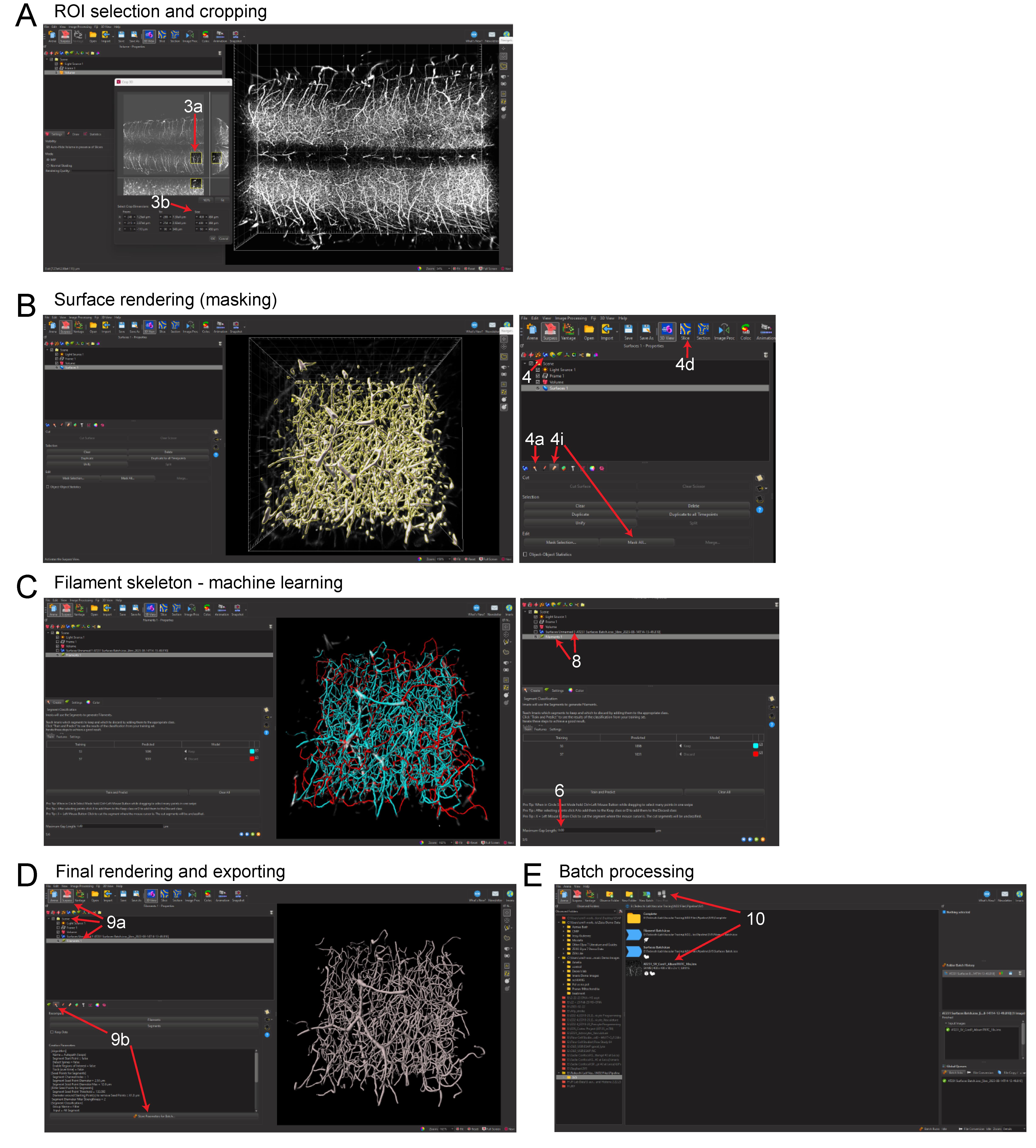
Figure 5. Imaris pipeline for convolutional reconstruction and analysis of vasculature networks in unsectioned organs and tissue specimens. (A) Region of interest (ROI) selection of the mouse spinal cord and three-dimensional cropping within Imaris. (B) Surface rendering (masking) step within Imaris. (C) Filament tracing machine learning step, showing predicted renderings of the spinal cord capillary network. (D) Completed three-dimensional rendering of the capillary network and steps for exporting object statistics and batch files. (E) Exporting statistics and editing batch files for multi-image batch processing.Select the leaf icon (sixth from the left) to begin filament tracing (Figure 5B).
Select Autopath (loops) no soma and no spine (Figure 5B).
Measure the diameter of the source channel within the Slice view as described in steps 4b and 4c.
Set the Source Channel to the newly created masked vasculature channel.
Select Multiscale seeding points and input the approximate diameter of the largest and smallest vessels using Slice view for measurement (Figure 5B).
Adjust the Seed Points Threshold to have seeding points populate the midline of desired vessels and reduce seeding points within the empty volume.
Note: Entering the slicer view may help to check the accuracy of seed point placement.
Seed points may need to be manually added or removed via Ctrl + left-click.
Classify seed points as either Keep or Discard depending on how they fill and match the vessel labeling. Use the circle selection tool on the right docked window to quickly select and classify groups of seed points.
Note: To keep selected points, press K; to discard them, press D (Figure 5B).
The size of the circle selection tool can be adjusted by holding Ctrl/Cmd + scroll on the mouse.
To select multiple points, hold Ctrl/Cmd + left-click/drag over the points you want to select. After enough seed points have been classified, select Train and Predict to begin training the machine learning algorithm.
Note: We have found a minimum of 50 classified points in each category is sufficient, although this will vary depending on the signal-to-noise ratio within the image.
Classify skeleton segments as Keep or Discard as described previously for step 5f–g.
Note: The algorithm tends to bridge parallel structures that are in proximity. Check high-density regions and classify them, as necessary. The Maximum Gap Length option also helps to mitigate this issue.
Filter the filament segments to correct for errors as described in step 5e (Figure 5C). We have found that filtering out segments with a length of less than 2–4 µm aids in correcting the bridging errors; however, this will vary between images.
Identify each layer (surface or filament) that will be exported with statistics with a unique identifier specific to the file and surface or filament being generated.
Critical: The default name for a surface created is “Surface 1.” Rename this to a unique ID for each surface or filament. If this step is not completed, statistics from multiple images cannot be exported.
Batch processing (Optional) (Figure 5C):
To save the new algorithm parameters within Surpass, select the desired surface or filament rendering under the Scene folder.
Note: Algorithm parameters for batch processing should be named, saved, and run individually for each rendering, e.g., save surface creation parameters as a separate batch file from filament tracing parameters and then sequentially run the batch processes on desired files.
Select the Creation (wand) button then Store Parameter For Batch Processing. This will create a batch process file within the same folder as the image that contains the algorithm.
In Arena, ensure the folder contains only the appropriate batch files and image files for batch processing. Right-click on the batch file and select Run.
To create a new algorithm within Arena, select Batch Process to open the algorithm wizard.
Select surfaces or filaments from the top left panel.
Drag and drop an image file to the open algorithm wizard pipeline and begin training.
Note: When training the algorithm for batch processing, ensure the channels and any masked channels are identical to the training file.
To save edits to the algorithm wizard, click on the save icon (floppy disk).
Critical: Edits made in the wizard do not save automatically. If the batch is started prior to saving changes, the algorithm wizard will use the batch file created since the last save, not since the last edit was made.
Export statistics via the Arena interface.
Select all images to be analyzed and select New Plot near the top of the window (Figure 5D). Each rendering with a unique name will be displayed here.
Ensure that only the renderings being exported with statistics are selected from the list (Figure 5D).
Change the displayed statistics by selecting the dropdown menu and scrolling to the desired statistic.
Note: Branch hierarchy is not an option due to the presence of looping structures.
Select the save icon (floppy disk) to export the statistics as a .xls file (Figure 5E).
FIJI/ImageJ reconstruction and analysis of vasculature networks in unsectioned organs and tissue specimens (Optional)
Note: The SNT plugin for FIJI/ImageJ must be downloaded and installed before beginning via the following link: https://imagej.net/update-sites/neuroanatomy.
Open FIJI/ImageJ and select File > Open (Figure 6A). Select the image that will be analyzed.
Optional: If the source signal is not white, convert the signal to binary by selecting Image > Adjust > Threshold.
Using the arrow buttons or manually, input a value to the right and adjust the top (minimum) threshold bar to find an acceptable level (Figure 6B). We have found that a value of roughly 80–110 (2.8%–3.6%) works, although this will vary between images.
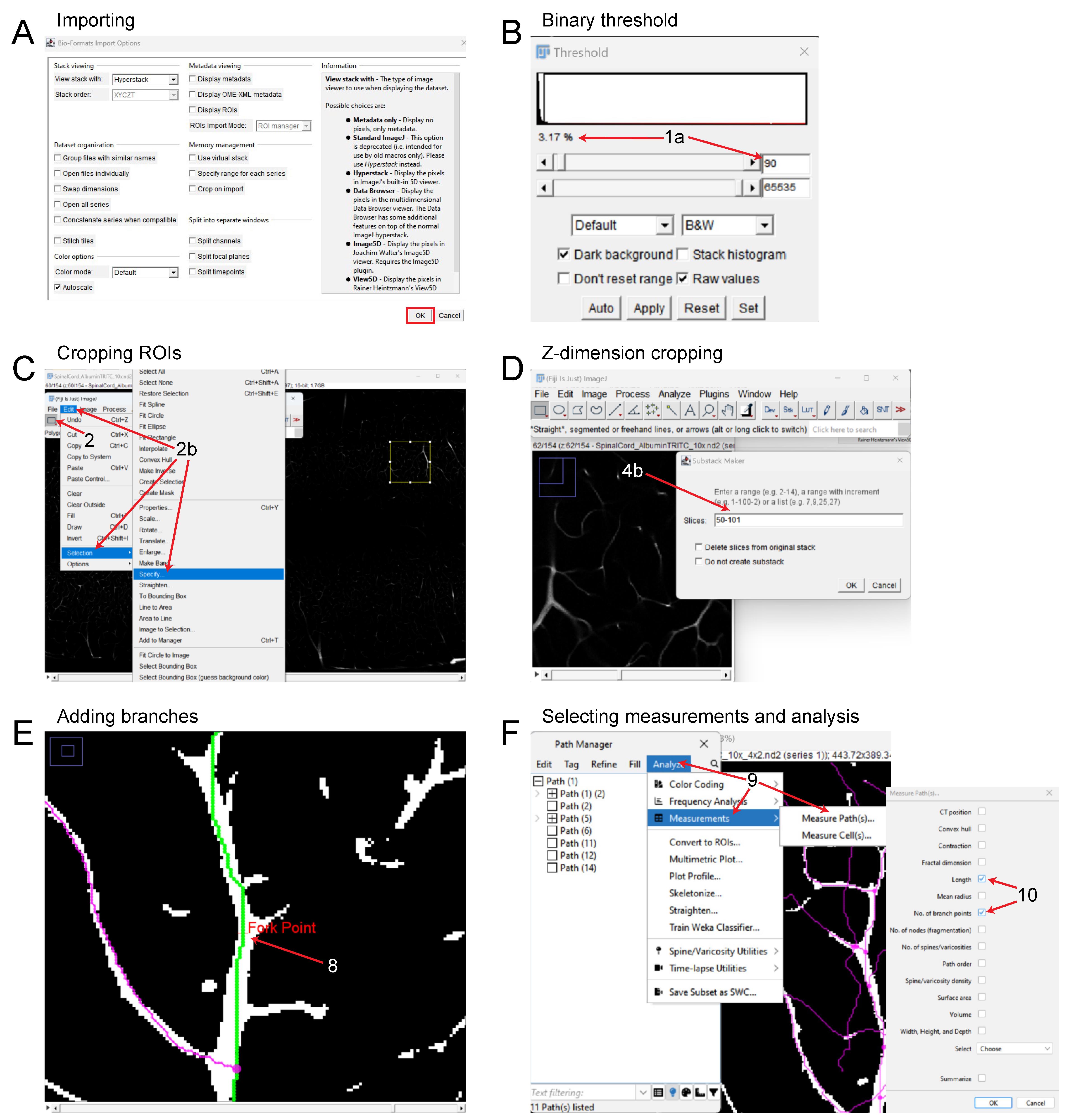
Figure 6. FIJI pipeline for reconstruction and analysis of vasculature networks in unsectioned organs and tissue specimens. (A) Importing 3D files into FIJI. (B) Adjusting binary threshold for improved visualization and tracing. (C) Setting a ROI and cropping the files in the x and y dimensions. (D) Cropping the image in the z dimension. (E) Tracing the vascular signal and adding branch points, depicting the Fork Point function. (F) Analyzing the vasculature and exporting statistics of interest.Determine a ROI within the image by selecting the rectangle tool under File (Figure 6C). Then, left-click and drag to the desired size.
The ROI can be precisely changed by manually inputting dimension parameters via Edit > Selection > Specify (Figure 6C).
Select Analyze > Tools > ROI Manager to save the current ROI selection.
Crop the current image selection via Image > Crop.
To crop a file in the z dimension, select Image > Hyperstacks > Make Subset….
Enter the range of stacks that will be traced (Figure 6D). Note that this distance in the z dimension will be related to the step size selected when imaging. (e.g., an image with 4 µm step size cropped to 50 stacks will be 200 µm in the z dimension).
Select Plugins > Neuroanatomy > SNT to begin tracing the vasculature.
Select the current image under the drop-down menu titled Image.
Begin tracing the vasculature by left-clicking on the image. It may be helpful to begin with a larger diameter vessel first to keep track of the tracings and branches.
Once two points are selected, click Y to keep or N to discard.
Repeat this process until the end of the signal is reached.
When finished with a path, press F to save and add it to the path manager.
Add branches as needed by pressing Alt + left-click (Figure 6E). Ensure the path that the branch will be coming off is selected by hovering the cursor over the path and pressing G. The selected path will be green.
Export statistics via the Path Manager window by selecting Analyze > Measurements > Measure Path(s) (Figure 6F).
From the new window, select Length and No of Branch Points (Figure 6F).
A new window will provide the specified parameters. Highlight these values, copy them, and paste them into an Excel spreadsheet.
Data analysis
The practicality and scalability of our protocol offer application across various fields of biomedical sciences. The entire procedure can be conducted by a competent graduate student or laboratory technician. Group size should be estimated using power analysis and historical laboratory data. Based on our experience, 6–7 biological replicates will produce robust and reproducible results. Examples of exclusion criteria include poor mouse perfusion, inconsistent vasculature tracing, tissue damage during dissection, or excessive photobleaching. Of note, three-dimensional reconstruction and analysis of vasculature networks using Imaris and ImageJ produced similar results (Table 2). A major limitation of ImageJ vs. Imaris is that it takes significantly longer to process the same ROI for three-dimensional reconstruction. Statistical analysis of albumin-TRITC-filled vasculature (Imaris pipeline) was performed using Prism (Version 10.0.1, GraphPad) through a Mann-Whitney test (Figure 7B). Other statistical analysis software (e.g., SPSS, R, or MATLAB) can also be used. For all analyses performed, significance was defined as p < 0.05. The exact value of biological replicates and the definition of measures are shown in the corresponding figure legend. Experimental data were evaluated blind to condition.
Table. 2 Imaris vs. FIJI comparison
| Imaris | FIJI | |
|---|---|---|
| Number of branch points | 78 | 52 |
| Total length (µm) | 5,778 | 5,642 |
Comparison of using Imaris vs. FIJI for vascular tracing and analysis using the same ROI with a mouse spinal cord sample.
Validation of protocol
To verify the robustness and reproducibility of our protocol, we compared results obtained by an experienced user (> 20 years of research experience) with those from a non-experienced user (e.g., a first-year graduate student with no prior experience in mouse perfusion, tissue clearing, three-dimensional imaging, and analysis). Our analysis demonstrated consistent and reproducible results between users (Figure 7). Additionally, this protocol has been already adopted in a previous publication (Tedeschi et al., 2022), which leveraged the vascular tracing methodology to assess capillary network changes following stroke in adult mice. A similar protocol has also been described in a previous study (Di Giovanna et al., 2018). Tissue clearing methods are adaptable and highly reproducible (Ueda et al., 2020). The clearing protocol we used here is based on the advanced CUBIC protocol for whole-brain and whole-body clearing and imaging (Susaki et al., 2015).
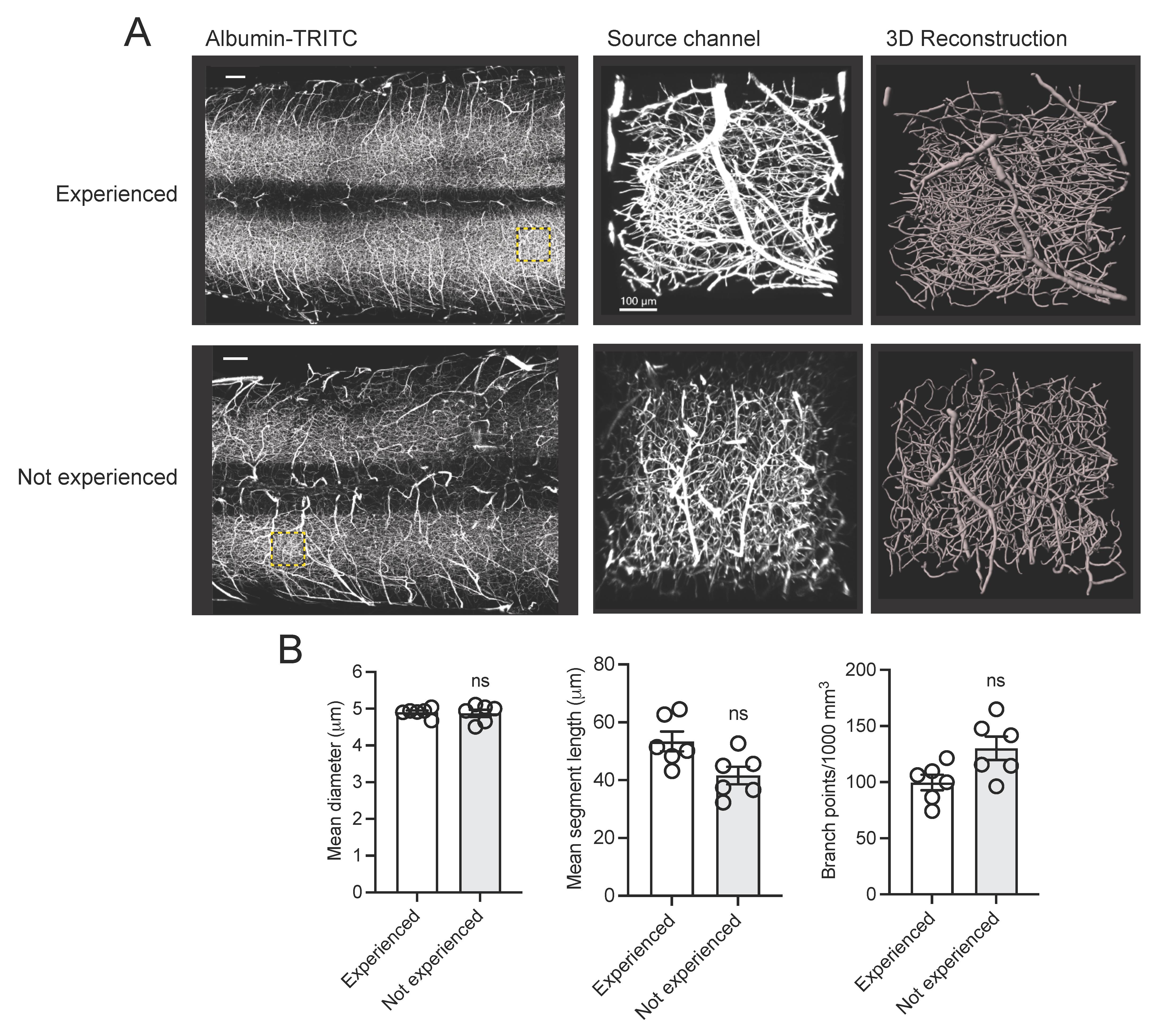
Figure 7. Assessing the robustness and reproducibility of our vasculature tracing, imaging, and analysis pipeline by compering results from users with and without research experience. (A) Representative fluorescence images of albumin-TRITC-filled vasculature networks in the adult mouse spinal cord. Regions of interest (ROIs) are depicted as a maximum intensity projection and three-dimensional renderings (Imaris). Scale bars: 200 µm. Data were generated by an experienced user (> 20 years research experience) and a non-experienced user (e.g., a first-year graduate student with no prior experience in mouse perfusion, tissue clearing, three-dimensional imaging, and analysis). (B) Quantification of (A). Mean and SEM (Mann-Whitney test, ns: not significant; n = 6 biological replicates/user).
General notes and troubleshooting
General notes
Although each component was chosen to achieve optimal image quality and precise quantification, modifications can be made to extend the utility of this protocol. The selection of a preconjugated fluorophore can be adapted to avoid spectral overlap in the instance of additional labeling strategies such as IHC or genetic reporters. When choosing a fluorophore, key molecular properties to be considered are excitation and emission spectra, quantum yield, and fluorescence lifetime. Check the specifics of your laser scanning microscope and confirm that the maximum excitation wavelength of the selected fluorophore is within the range accepted by your imaging system. Our chosen fluorophore, TRITC, has a comparatively high quantum yield and fluorescence lifetime, while its excitation spectrum responds to red-shifted light, peaking at 544 nm. This component is crucial, as longer wavelengths are less likely to be attenuated in thick samples, providing improved signal-to-noise ratio and deeper imaging of samples (Belov et al., 2010; Im et al., 2019). Optical clearing methodologies can be adjusted to improve transparency with particular tissue compositions. The decision to use aqueous-based vs. organic solvent–based clearing methods will primarily depend on tissue thickness and composition, although some clearing methods can damage the fluorophore and should be carefully assessed. Additionally, these two classifications of tissue clearing have several variations of protocols that can be tailored to the research question at hand. Imaging offers a variety of suitable microscopy strategies including 1P and 2P laser scanning and light sheet fluorescence microscopy (Hilton et al., 2019; Tedeschi et al., 2016 and 2022; Wang et al., 2018). Lastly, three-dimensional reconstruction can be completed using either Imaris or ImageJ. Note that a benefit of ImageJ is that it is a free, open-source software and less computationally demanding. This can be leveraged for less dense vascular networks, such as those found in peripheral nerves (e.g., facial or sciatic nerves).
Further adaptations of this protocol permit the study of blood–brain barrier/blood–spinal cord barrier (BBB/BSCB) integrity in CNS injury (e.g., stroke, traumatic brain, and spinal cord injury) or disease (e.g., Alzheimer’s disease, multiple sclerosis, etc.) models. To trace vessels, we leveraged a 67 kDa albumin-fluorophore conjugate in a 2% gelatin mixture. At this molecular weight, the conjugate cannot leak out of intact capillaries but can be used to identify compromised barrier regions by adjusting the concentration of gelatin. Decreasing the percentage of gelatin to approximately 0.5% will reduce viscosity, allowing albumin-TRITC to leak through compromised regions and illustrate the extent of BBB/BSCB damage in vivo. While this is possible with other vessel tracing methods, our pipeline offers the advantage of quantitatively assessing concurrent changes in other capillary network characteristics that can accompany a loss of barrier integrity.
Troubleshooting
Table 3. Troubleshooting
| Problem observed | Possible cause | Solution |
| Poor, uneven, or absence of fluorescence during image acquisition | Sub-optimal perfusion or fluorophore damaged during preparation |
|
| High background/noise during image acquisition | Clearing incubation time too short, samples too thick, or improper clearing method for sample |
|
| Imaris not showing files in Arena | Overloaded cache |
|
| Imaris frequently crashing/not responding | Files too large or computer specifications not sufficient |
|
| ||
| ||
| Unable to connect gaps in signal during FIJI/ImageJ tracing | Cursor auto-snapping enabled |
|
Acknowledgments
We would like to thank Dr. Wenjing Sun for critically reading and all members of the laboratory for discussion. This work was supported by the National Institute of Neurological Disorders (grant R01NS110681).
Competing interests
All authors declare no competing interests.
Ethical considerations
The methods and experimental procedures described above are designed to limit discomfort and distress to the animals that may affect the interpretation of the results. All experiments were performed following protocols approved by the Institutional Animal Care and Use Committee at The Ohio State University (Protocol #2017A00000027-R2) and complied with accepted ethical best practices.
References
- Belov, V. N., Wurm, C. A., Boyarskiy, V. P., Jakobs, S. and Hell, S. W. (2010). Rhodamines NN: a novel class of caged fluorescent dyes. Angew Chem Int Ed Engl 49(20): 3520–3523. https://doi.org/10.1002/anie.201000150
- Cheung, K. C. P., Fanti, S., Mauro, C., Wang, G., Nair, A. S., Fu, H., Angeletti, S., Spoto, S., Fogolari, M., Romano, F., et al. (2020). Preservation of microvascular barrier function requires CD31 receptor-induced metabolic reprogramming. Nat Commun 11(1): 3595. https://doi.org/10.1038/s41467-020-17329-8
- Di Giovanna, A. P., Tibo, A., Silvestri, L., Mullenbroich, M. C., Costantini, I., Allegra Mascaro, A. L., Sacconi, L., Frasconi, P. and Pavone, F. S. (2018). Whole-Brain Vasculature Reconstruction at the Single Capillary Level. Sci Rep 8(1): 12573. https://doi.org/10.1038/s41598-018-30533-3
- Evans, C. E., Iruela-Arispe, M. L. and Zhao, Y. Y. (2021). Mechanisms of Endothelial Regeneration and Vascular Repair and Their Application to Regenerative Medicine. Am J Pathol 191(1): 52–65. https://doi.org/10.1016/j.ajpath.2020.10.001
- Felmeden, D. C., Blann, A. D. and Lip, G. Y. (2003). Angiogenesis: basic pathophysiology and implications for disease. Eur Heart J 24(7): 586–603. https://doi.org/10.1016/s0195-668x(02)00635-8
- Hilton, B. J., Blanquie, O., Tedeschi, A. and Bradke, F. (2019). High-resolution 3D imaging and analysis of axon regeneration in unsectioned spinal cord with or without tissue clearing. Nat Protoc 14(4): 1235–1260. https://doi.org/10.1038/s41596-019-0140-z
- Im, K., Mareninov, S., Diaz, M. F. P. and Yong, W. H. (2019). An Introduction to Performing Immunofluorescence Staining. Methods Mol Biol 1897: 299–311. https://doi.org/10.1007/978-1-4939-8935-5_26
- Marien, K. M., Croons, V., Waumans, Y., Sluydts, E., De Schepper, S., Andries, L., Waelput, W., Fransen, E., Vermeulen, P. B., Kockx, M. M. et al. (2016). Development and Validation of a Histological Method to Measure Microvessel Density in Whole-Slide Images of Cancer Tissue. PLoS One 11(9): e0161496. https://doi.org/10.1371/journal.pone.0161496
- Menozzi, L., Del Aguila, A., Vu, T., Ma, C., Yang, W. and Yao, J. (2023). Three-dimensional non-invasive brain imaging of ischemic stroke by integrated photoacoustic, ultrasound and angiographic tomography (PAUSAT). Photoacoustics 29: 100444. https://doi.org/10.1016/j.pacs.2022.100444
- Ostergaard, L., Engedal, T. S., Moreton, F., Hansen, M. B., Wardlaw, J. M., Dalkara, T., Markus, H. S. and Muir, K. W. (2016). Cerebral small vessel disease: Capillary pathways to stroke and cognitive decline. J Cereb Blood Flow Metab 36(2): 302–325. https://doi.org/10.1177/0271678X15606723
- Pac, J., Koo, D. J., Cho, H., Jung, D., Choi, M. H., Choi, Y., Kim, B., Park, J. U., Kim, S. Y. and Lee, Y. (2022). Three-dimensional imaging and analysis of pathological tissue samples with de novo generation of citrate-based fluorophores. Sci Adv 8(46), eadd9419. https://doi.org/10.1126/sciadv.add9419
- Rust, R., Kirabali, T., Gronnert, L., Dogancay, B., Limasale, Y. D. P., Meinhardt, A., Werner, C., Lavina, B., Kulic, L., Nitsch, R. M. et al. (2020). A Practical Guide to the Automated Analysis of Vascular Growth, Maturation and Injury in the Brain. Front Neurosci 14: 244. https://doi.org/10.3389/fnins.2020.00244
- Susaki, E. A., Tainaka, K., Perrin, D., Yukinaga, H., Kuno, A. and Ueda, H. R. (2015). Advanced CUBIC protocols for whole-brain and whole-body clearing and imaging. Nat Protoc 10(11): 1709–1727. https://doi.org/10.1038/nprot.2015.085
- Tedeschi, A., Dupraz, S., Laskowski, C. J., Xue, J., Ulas, T., Beyer, M., Schultze, J. L. and Bradke, F. (2016). The Calcium Channel Subunit Alpha2delta2 Suppresses Axon Regeneration in the Adult CNS. Neuron 92(2): 419–434. https://doi.org/10.1016/j.neuron.2016.09.026
- Tedeschi, A., Larson, M. J. E., Zouridakis, A., Mo, L., Bordbar, A., Myers, J. M., Qin, H. Y., Rodocker, H. I., Fan, F., Lannutti, J. J. et al. (2022). Harnessing cortical plasticity via gabapentinoid administration promotes recovery after stroke. Brain 145(7): 2378–2393. https://doi.org/10.1093/brain/awac103
- Ueda, H. R., Erturk, A., Chung, K., Gradinaru, V., Chedotal, A., Tomancak, P. and Keller, P. J. (2020). Tissue clearing and its applications in neuroscience. Nat Rev Neurosci 21(2): 61–79. https://doi.org/10.1038/s41583-019-0250-1
- Wang, Z., Maunze, B., Wang, Y., Tsoulfas, P. and Blackmore, M. G. (2018). Global Connectivity and Function of Descending Spinal Input Revealed by 3D Microscopy and Retrograde Transduction. J Neurosci 38(49): 10566-10581. https://doi.org/10.1523/JNEUROSCI.1196-18.2018
- Xiong, B., Li, A., Lou, Y., Chen, S., Long, B., Peng, J., Yang, Z., Xu, T., Yang, X., Li, X. et al. (2017). Precise Cerebral Vascular Atlas in Stereotaxic Coordinates of Whole Mouse Brain. Front Neuroanat 11: 128. https://doi.org/10.3389/fnana.2017.00128
Article Information
Copyright
© 2024 The Author(s); This is an open access article under the CC BY-NC license (https://creativecommons.org/licenses/by-nc/4.0/).
How to cite
Vidman, S., Dion, E. and Tedeschi, A. (2024). A Versatile Pipeline for High-fidelity Imaging and Analysis of Vascular Networks Across the Body. Bio-protocol 14(4): e4938. DOI: 10.21769/BioProtoc.4938.
Category
Neuroscience > Neuroanatomy and circuitry > Fluorescence imaging
Cell Biology > Tissue analysis > Tissue imaging
Do you have any questions about this protocol?
Post your question to gather feedback from the community. We will also invite the authors of this article to respond.