- Protocols

- Articles and Issues
- For Authors
- About
- Become a Reviewer

Protein Level Quantification Across Fluorescence-based Platforms
Published: Vol 13, Iss 19, Oct 5, 2023 DOI: 10.21769/BioProtoc.4834 Views: 2033
Reviewed by: Anonymous reviewer(s)
Original research article
The authors used this protocol in:
Feb 2022

Protocol Collections
Comprehensive collections of detailed, peer-reviewed protocols focusing on specific topics


Abstract
Biological processes are dependent on protein concentration and there is an inherent variability among cells even in environment-controlled conditions. Determining the amount of protein of interest in a cell is relevant to quantitatively relate it with the cells (patho)physiology. Previous studies used either western blot to determine the average amount of protein per cell in a population or fluorescence intensity to provide a relative amount of protein. This method combines both techniques. First, the protein of interest is purified, and its concentration determined. Next, cells containing the protein of interest with a fluorescent tag are sorted into different levels of intensity using fluorescence-activated cell sorting, and the amount of protein for each intensity category is calculated using the purified protein as calibration. Lastly, a calibration curve allows the direct relation of the amount of protein to the intensity levels determined with any instrument able to measure intensity levels. Once a fluorescence-based instrument is calibrated, it is possible to determine protein concentrations based on intensity.
Key features
• This method allows the evaluation and comparison of protein concentration in cells based on fluorescence intensity.
• Requires protein purification and fluorescence-activated cell sorting.
• Once calibrated for one protein, it allows determination of the levels of this protein using any fluorescence-based instrument.
• Allows to determine subcellular local protein concentration based on combining volumetric and intensity measurements.
Graphical overview
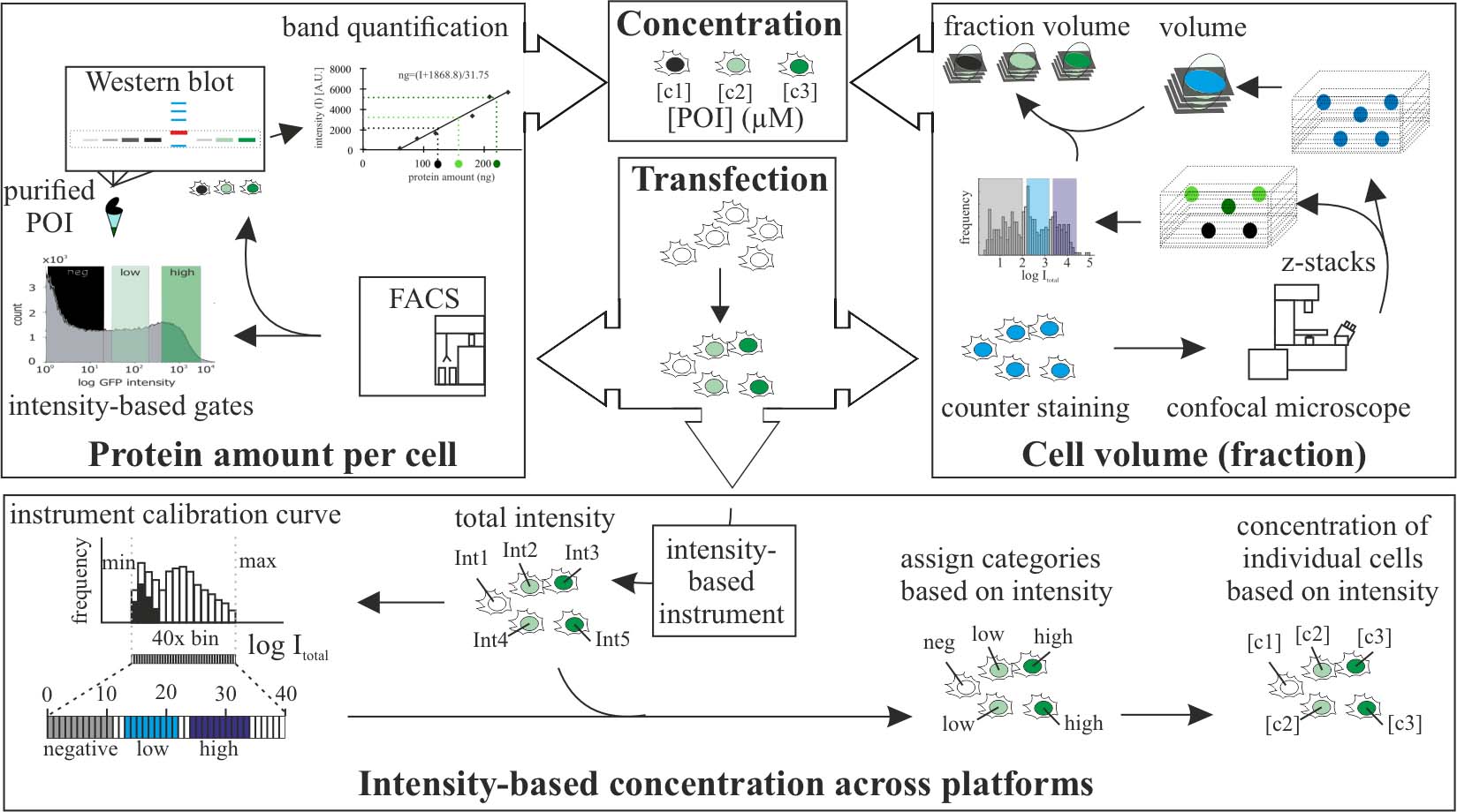
Protein level quantification across fluorescence-based platforms
Background
The use of fluorescently tagged proteins is a common tool in cell biology to study a variety of molecular processes. Although fluorescence is directly related to concentration of the fluorophore, the values of intensities do not translate directly into concentration of molecules. This is important to reproduce (patho)physiological concentrations of molecules including proteins. Western blots can be used to determine the average amount of proteins within a cell population. We performed fluorescence-activated cell sorting (FACS) prior to analysis by western blot to quantify protein levels within a cell population with defined fluorescence intensities and cell amounts. In addition, we developed a method that allows the direct relation of fluorescence intensities to get molecular concentration categories at the single-cell level. Furthermore, we expanded the method to allow concentration comparison between samples detected in different systems. Lastly, we extended the method to calculate average subcellular concentration variations. Other existing methods to determine protein concentrations are based on single-molecule imaging to calculate the number of molecules in beads (Chiu et al., 2001; Sugiyama et al., 2005) or, alternatively, use lipid or polymer layers in which the density of the fluorophore is known (Dustin, 1997; Zwier et al., 2004; Galush et al., 2008). These methods, although maybe more accurate in the estimation of concentration than ours, require calibration for each experiment and/or sophisticated equipment, whereas our method relies on equipment available in most molecular cell biology laboratories.
In the publication in which we utilized the method (Zhang et al., 2022), we used it to quantify ectopic protein concentrations in single cells and subcellular compartments. This allowed us to reproduce the same concentrations in cells and in in vitro experiments and to relate it to physiological tissue concentrations. Variations of the method can be used to quantify endogenous levels of tagged proteins (i.e., in cells with genomically engineered loci) or proteins labeled with antibodies.
Materials and reagents
Biological samples
Bovine serum albumin (BSA) (Sigma-Aldrich, catalog number: A8412); see General note 1
C2C12, mouse (Mus musculus) myoblasts (Yaffe and Saxel, 1977); see General note 1
Plasmid pc1208 (pEG-MeCP2) (Kudo et al., 2003); see General note 1
Rat IgG anti-MeCP2 4H7 antibody. Self-made, not commercial (Jost et al., 2011); see General note 1
Donkey anti-rat IgG-Cy3 antibody (Jackson ImmunoResearch, catalog number: 111560); see General notes 1 and 2
Reagents
1,4-Diazabicyclo-[2.2.2]octane (DABCO) (Sigma-Aldrich, catalog number: D2522)
2-propanol (AppliChem GmbH, catalog number: 131090.1212)
4′,6′-diamidine-2-phenylindole dihydrochloride (DAPI) (Carl Roth, catalog number: 6335.1)
Aluminum sulfate 14–18 hydrate (Carl Roth, catalog number: 3731.1)
Ammonium persulfate (Carl Roth, catalog number: 9592.3)
Bromophenol blue (Bio-Rad Laboratories, catalog number: 161-0404)
Coomassie, Brilliant Blue R (Sigma-Aldrich, catalog number: 1.12553)
Dimethylsulfoxide (DMSO) (Sigma-Aldrich, catalog number: D4540)
Di-sodium hydrogen phosphate 7-hydrate (Na2HPO4·7H2O) (Carl Roth, catalog number: X987.2)
Dithiothreitol (DTT) (Sigma-Aldrich, catalog number: D9779)
Ethanol absolute pure, pharma grade (AppliChem GmbH, catalog number: A4230)
Ethylenedinitrilotetraacetic acid (EDTA) (AppliChem GmbH, catalog number: 131026.1211)
Glucose (Sigma-Aldrich, catalog number: G5400)
Glycerol (Sigma-Aldrich, catalog number: G9422)
Hybond ECL membrane (nitrocellulose membrane) (VWR, catalog number: RPN3032D)
Low fat milk pulver (Sucofin)
Methanol for analysis EMPARTA® ACS (Sigma Aldrich, catalog number: 1070182511)
Mowiol® 4-88 (Sigma-Aldrich, catalog number: 81381)
NonidetTM P-40 substitute (NP-40) (Roche, catalog number: 11332473001)
Pepstatin A (Sigma-Aldrich, catalog number: P5318)
Phenylmethylsulfonyl fluoride (PMSF) (Carl Roth, catalog number: 6367.1)
Potassium chloride (KCl) (Sigma-Aldrich, catalog number: P9541)
Potassium dihydrogen phosphate (KH2PO4) (Carl Roth, catalog number: 3904.1)
Tris (Sigma-Aldrich, catalog number: 93362)
Sodium chloride (NaCl) (Carl Roth, catalog number: 3957.1)
Sodium dodecyl sulfate (SDS) (Sigma-Aldrich, catalog number: 11667289001)
Trans-epoxysuccinyl-L-leucylamido(4-guanidino)butane (E64) (Sigma-Aldrich, catalog number: E3132)
Tween 20 (Carl Roth, catalog number: 131026.1211)
Whatman 3MM CHR (Whatman paper) (Cytiva, catalog number: 3030-672)
Solutions
Acrylamide/bis-acrylamide 30% (Polyacrylamide) (Sigma-Aldrich, catalog number: A3699)
Dulbecco’s modified Eagle’s medium, high glucose (Sigma-Aldrich, catalog number: D7777)
Fetal bovine serum advanced (Capricorn Scientific, catalog number: FBS-11A)
Formaldehyde solution, 36.5%–38% in H2O (Sigma-Aldrich, catalog number: F8775)
Orthophosphoric acid (Carl Roth, catalog number: 6366.1)
PierceTM 660 nm Protein Assay Reagent (Thermo Fisher, catalog number: 22660)
PierceTM 10× Western Blot Transfer buffer, methanol-free (transfer buffer) (Thermo Fisher, catalog number: 35040)
Tetramethylethylenediamine (TEMED) (Sigma-Aldrich, catalog number: T9281)
Trypsin (Sigma-Aldrich, catalog number: T4049)
Ammonium persulfate 10% (see Recipes)
Coomassie destaining solution (see Recipes)
Coomassie staining solution (see Recipes)
DAPI solution (see Recipes)
E64 solution (see Recipes)
Loading buffer (see Recipes)
Low-fat milk 3% in PBS (see Recipes)
Low-fat milk 5% in PBS (see Recipes)
Lysis buffer (see Recipes)
Mounting media (see Recipes)
Pepstatin A solution (see Recipes)
Phosphate buffered saline (PBS) (see Recipes)
PBS-EDTA 0.02% (w/v) (see Recipes)
PMSF solution (see Recipes)
Polyacrylamide gel 5% (stacking) for 10 mL gel (see Recipes)
Polyacrylamide gel 8% (separating) for 10 mL gel (see Recipes)
Running buffer 10× (see Recipes)
Sodium dodecyl sulfate (SDS) 10% (see Recipes)
Tris 1 M pH 6.8 (see Recipes)
Tris 1 M pH 8.5 (see Recipes)
Tris 1.5 M pH 8.8 (see Recipes)
Recipes
Ammonium persulfate 10%
Reagent Final concentration Quantity Ammonium persulfate 10% (w/v) 1 g H2O n/a to 10 mL Total n/a 10 mL Coomassie destaining solution
Reagent Final concentration Quantity Ethanol 10% (v/v) 40 mL Orthophosphoric acid 2% (v/v) 2 mL H2O n/a 58 mL Total n/a 100 mL Coomassie staining solution
Reagent Final concentration Quantity Coomassie 0.2% (w/v) 0.2 g Orthophosphoric acid 2% (v/v) 2 mL Ethanol 10% (v/v) 10 mL H2O n/a to 100 mL Total n/a 100 mL DAPI solution
Reagent Final concentration Quantity DAPI 1 mg/mL 10 mg H2O n/a to 10 mL Total n/a 10 mL E64 solution
Reagent Final concentration Quantity E64 1 mM 360 μg Ethanol 50% (v/v) 500 μL H2O n/a 500 μL Total n/a 1 mL Loading buffer
Reagent Final concentration Quantity Tris 50 mM 0.3 g SDS 2% (v/v) 2 mL Glycerol 10% (v/v) 10 mL Bromophenol blue 0.01% (v/v) 100 μL DTT 100 mM 1.5 g H2O n/a to 100 mL Total n/a 100 mL Low-fat milk 3% in PBS
Reagent Final concentration Quantity Low-fat milk pulver 3% (w/v) 0.3 g PBS n/a to 10 mL Total n/a 10 mL Low-fat milk 5% in PBS
Reagent Final concentration Quantity Low-fat milk pulver 3% (w/v) 0.5 g PBS n/a to 10 mL Total n/a 10 mL Lysis buffer
Reagent Final concentration Quantity Tris 25 mM 0.03 g NaCl 1 M 0.6 g Glucose 50 mM 0.09 g EDTA 10 mM 0.03 g Tween 20 0.2% (v/v) 20 μL NonidetTM P-40 substitute 0.2% (v/v) 20 μL PMSF solution 1 mM 1 μL E64 solution 10 μM 1 μL Pepstatin A solution 29 μM 1 μL H2O n/a 10 mL Total n/a 10 mL Mounting media
Reagent Final concentration Quantity Mowiol 4-88 13% (w/v) 8 g Tris-HCl 1 M pH 8.5 133 mM 8 mL H2O n/a 32 mL Glycerol 33% (v/v) 20 mL DABCO 2% (w/v) 1.2 g Total n/a 60 mL Add mowiol to Tris and H2O and heat to 50–60 °C while stirring.
Cool down to room temperature.
Add glycerol and stir again.
Add DABCO and dissolve it by stirring.
Spin the solution at 5,000× g for 15 min.
Aliquot the supernatant and store at -20 °C.
Pepstatin A solution
Reagent Final concentration Quantity Pepstatin A 2.9 mM 2 mg DMSO n/a 1 mL Total n/a 1 mL Phosphate buffered saline (PBS)
Reagent Final concentration Quantity NaCl 1.37 M 80 g KCl 27 mM 2 g Na2HPO4·7H2O 10 mM 21.7 g KH2PO4 10 mM 2.4 g H2O n/a to 1 L Total n/a 1 L PBS-EDTA 0.02% (w/v)
Reagent Final concentration Quantity EDTA 0.02 % (w/v) 2 mg PBS n/a to 100 mL Total n/a 100 mL PMSF solution
Reagent Final concentration Quantity PMSF 100 mM 17.42 mg 2-propanol n/a 1 mL Total n/a 1 mL Polyacrylamide gel 5% (stacking) for 10 mL gel
Reagent Final concentration Quantity Polyacrylamide 5% (v/v) 0.33 mL Tris 1 M pH 6.8 125 mM 0.25 mL SDS 10% 0.1% (v/v) 0.02 mL Ammonium persulfate 10% 0.1% (v/v) 0.02 mL TEMED 0.001% (v/v) 0.002 mL H2O n/a 1.4 mL Total n/a 2 mL Polyacrylamide gel 8% (separating) for 10 mL gel (see General note 1)
Reagent Final concentration Quantity Polyacrylamide 8% (v/v) 2.7 mL Tris 1.5 M pH 6.8 375 mM 2.5 mL SDS 10% 0.1% (v/v) 0.1 mL Ammonium persulfate 10% 0.1% (v/v) 0.1 mL TEMED 0.0006% (v/v) 0.006 mL H2O n/a 4.6 mL Total n/a 10 mL Running buffer 10×
Reagent Final concentration Quantity Tris base 25 mM 30 g Glycin 1.92 M 144 g SDS 1% (v/v) 100 mL H2O n/a to 1 L Total n/a 1 L SDS 10%
Reagent Final concentration Quantity SDS 10% (v/v) 10 mL H2O n/a 90 mL Total n/a 100 mL Tris 1 M pH 6.8
Reagent Final concentration Quantity Tris 1 M 12.1 g H2O n/a to 100 mL Total n/a 100 mL Tris 1 M pH 8.5
Reagent Final concentration Quantity Tris 1 M 12.1 g H2O n/a to 100 mL Total n/a 100 mL Tris 1.5 M pH 8.8
Reagent Final concentration Quantity Tris 1.5 M 18.15 g H2O n/a to 100 mL Total n/a 100 mL
Equipment
AMAXA nucleofector (Lonza) or equivalent. Required for transfection of cells. See General note 1
Confocal microscope Leica TCS SPE-II (Leica) or equivalent. Required for imaging z-stacks to calculate volumes. See General note 1
Imager AI600 (Amersham) or equivalent. Required for imaging of SDS-PAGE gels (Epi-white light of 470–635 nm, any appropriate filter to see Coomassie stained proteins) and western blots (fluorescence epi light: 460, 520, or 630 nm with corresponding emission filters Cy2-525BP20, Cy3-605BP40, or Cy5-705BP40, see General note 2)
Mini-PROTEAN Tetra Vertical Electrophoresis Cell (Bio-Rad Laboratories) or equivalent
PowerPac Basic Power Supply (Bio-Rad Laboratories) or equivalent
S3e Cell Sorter (Bio-Rad Laboratories) or equivalent. It requires an illumination source and filters fitting to the fluorescent tag fused to the protein of interest: for EGFP, a 488 nm laser with emission filter 525/30 nm can be used
Single-molecule setup on a Nikon Eclipse Ti (Nikon). Used as example of fluorescence platforms. In the example given, EGFP images were taken using an OBIS 488 nm (100 mW) laser and a Quadbandpass (432/25 515/25 595/25 730/70 nm) filter from Nikon. See General note 1
Trans-Blot® SD Semi-Dry Transfer Cell (Bio-Rad Laboratories) or equivalent
Wide field microscope Axiovert 200 (Zeiss). Used as example of fluorescence platforms. In the example given, EGFP images were taken using a HBO100 bulb and a hard coated EGFP filter (ex: 482/18; bs: 495LP; em: 520/28). See General note 1
12 mm round coverslips (thickness 0.13–0.16 mm) (Diagonal, catalog number 41001112) or equivalent according to your microscope sample
#1.5H 24 mm round coverslips (thickness 175 ± 5 μm) (Thor laboratories, catalog number: CG15XH1). Used for live-cell microscopy in single-molecule setup. See General note 1
Widefield microscope Nikon Eclipse TiE2 (Nikon). Used for validation of the gate sorting across platforms. Spectra X LED 395 ± 25 nm (295 mW) and 370 ± 24 nm were used as illumination for DAPI and GFP respectively and a Quadbandpasss (432 ± 25, 515 ± 25, 595 ± 25, 730 ± 70 nm) as emission filter. Images were acquired using a 20× SPlan Fluor LWD DIC objective with numerical aperture of 0.7
Software and datasets
S3 ProSortTM Software (Bio-Rad Laboratories) or equivalent. Used to analyze and sort the cells in the cell sorter
ImageJ (FIJI) (Schindelin et al., 2012). In the examples given, FIJI version 1.52q was used and the plugin BioFormats was required to open the images generated in the widefield and confocal microscopes
Volocity 6.3 (Perkin-Elmer). See General note 1. ImageJ plugin 3D suite can be used instead to calculate volumes and intensity in z-stacks
Procedure
Protein purification and concentration validation by SDS-polyacrylamide gel electrophoresis (PAGE)
Purify the protein. You will need a purified version of the protein of interest (POI) that you want to study. It can be either untagged or tagged (see General note 3). Due to the many possibilities in protein purification, we will not include a description of the protein purification that we used, which can be found in the manuscript (Zhang et al., 2022).
Analyze the purified protein using SDS-PAGE.
Prepare dilutions with known quantities (250, 500, 750, 1,000, 1,500, 2,000 ng) of a reference protein (i.e., BSA) for a final volume of 15 μL in H2O.
Estimate the concentration of the purified protein by a colorimetric assay (e.g., PierceTM 660 nm Protein Assay Reagent).
Prepare specific quantities of the purified protein using the estimations (400, 600, 800, 1,000 ng) to a final volume of 15 μL in H2O.
Mix the dilutions of reference protein with 5 μL of loading buffer 4× to a final concentration 1×, boil them in 95 °C for 5 min, and then keep on ice.
Mix the different quantities of purified protein with 5 μL of loading buffer 4× to a final concentration 1×, boil them at 95 °C for 5 min, and then keep on ice.
Place a polyacrylamide gel in the electrophoresis chamber and fill it with 1× running buffer.
Analyze the samples by polyacrylamide gel electrophoresis with constant 100 V.
Incubate the gel in Coomassie staining solution overnight (~16 h).
Incubate the gel in destaining solution (2× 10 min) and equilibrate in H2O.
Image the gel in the imager (Figure 1A).
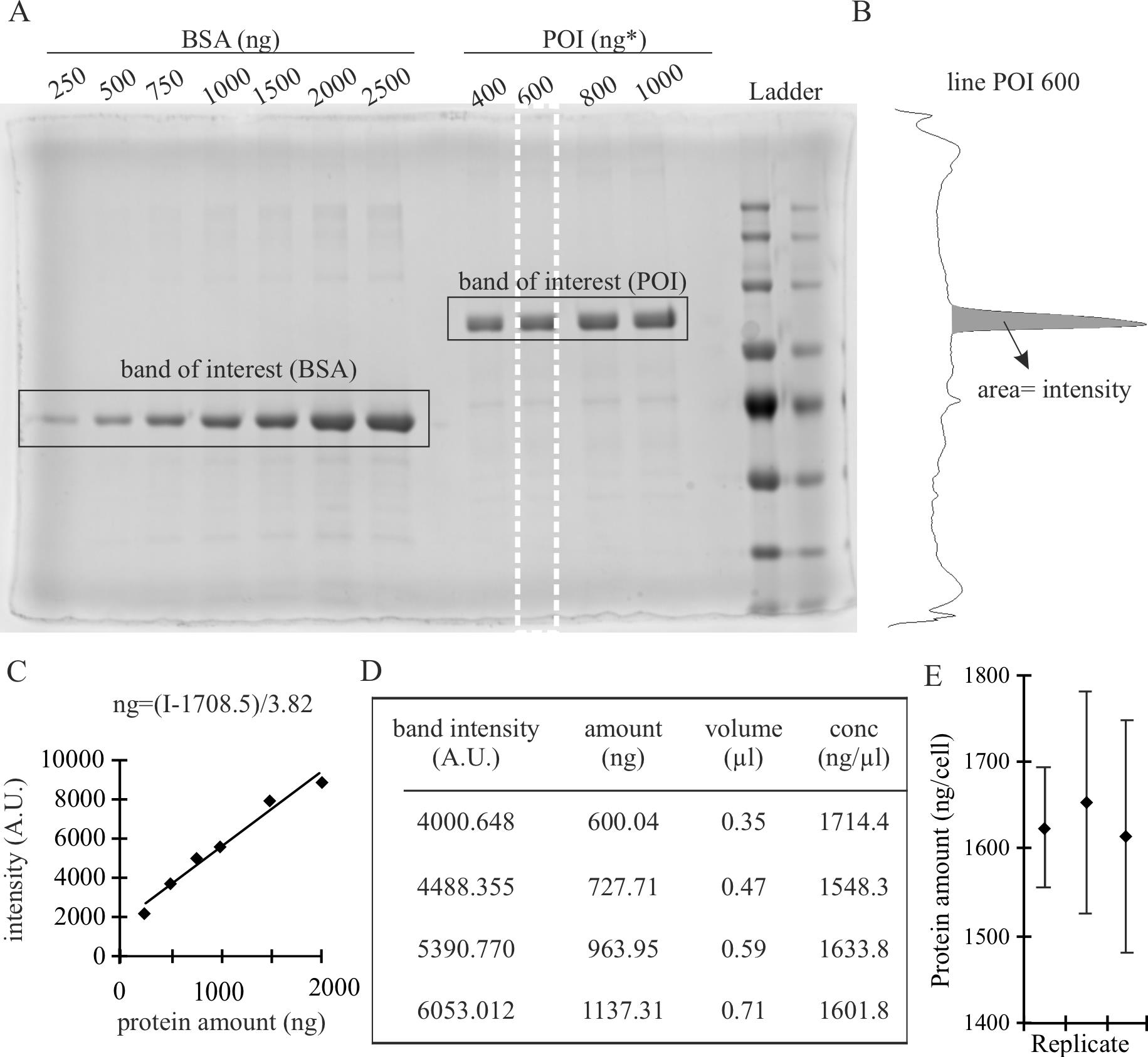
Figure 1. SDS-PAGE stained with Coomassie and analysis to validate the concentration of the purified protein. (A) Example of gel for validation. Known quantities of bovine serum albumin (BSA) are loaded together with different quantities of purified protein of interest (POI) estimated by colorimetric assay. Modified from Zhang et al. (2022). The white dashed line represents the selection used for quantification in B. (B) Intensity profile obtained in ImageJ using the gel analysis tool. Selections of the width of the band were done for individual bands and the area of the band of interest was calculated as the area under the peak. (C) Calibration curve based on the intensity measures obtained in B. The equation of the regression curve is described within the graph. (D) Calculations to obtain the corrected concentration (conc) of the POI, based on the intensity measurements of the POI bands using the equation of the regression curve from B, allow the determination of the corrected amount of POI from the calculated intensity of the band and the concentration in ng/μL as the average from the values obtained, 1624.6 ± 80.3 ng/μL. The values displayed are the calculation from left (POI 400 ng) to right (POI 1000) in the gel shown in A. The calculation of the error is described in the section data analysis. (E) Measurements and standard deviations for three technical replicates, each of them taking four band intensities to calculate the average as shown in D (which corresponds to left replicate).
Validate the concentration of purified protein by image analysis of the gel using ImageJ.
Generate a rectangular selection that covers a complete band.
Create a region of interest using the function Analyze → Gels → Select First Lane (for the first lane) and Analyze → Gels → Select Next Lane (for the others) (Figure 1A, white dashed line).
Get the intensity measurements using the function Analyze → Gels → Plot Lanes (Figure 1B).
Quantify the intensity of the bands as the area under the peak (Figure 1B). To do so: i) draw a horizontal lane in the base of the peak using the tool straight line so the peak is closed; ii) use the tool wand to select the peak; iii) automatically, it will display the area of the region selected.
Plot the intensity (area) against the known concentration of the reference protein and generate a regression curve (Figure 1C).
The equation of the regression curve is Y = a × X + b, being X the quantity of protein (in ng) and Y the intensity. Therefore, considering X = (Y - b)/a, you can calculate the protein amount based on intensity (Figure 1C). The parameter b corresponds to the background of the specific gel.
Use the intensity values obtained from the area under the peaks for each estimated amount of POI to get the actual values (Figure 1D).
You can get the concentration of the POI by dividing the amount of POI by the volume from the original solution added in each well (Figure 1D). The concentration of POI is the average of these values.
Calculation of protein amounts in cell fractions using fluorescence activated cell sorting and western blot
Sample preparation: grow the cells in the specific conditions required for its culture. You will need 106–107 cells in a 10 cm cell culture plate from wildtype (untransfected cells) and transfected cells. This step should be adapted to the specific cell line used. In the case of C2C12 using AMAXA electroporation:
Seed 50 cells/cm2 in a 10 cm cell culture plate.
Grow overnight in growth media at 37 °C with 5% CO2.
Remove media.
Wash cells with PBS-EDTA.
Add 2 mL of trypsin.
Incubate for 5 min at 37 °C.
Stop the trypsin with 4 mL of growth media.
Seed 0.5 mL of cells into a new 10 cm cell culture plate with 9 mL of growth media (untransfected sample).
Centrifuge 1 mL of cells at 0.3× g for 5 min and discard the supernatant.
Mix 2–5 μg of plasmid in 100 μL of room-temperature AMAXA M1 solution.
Resuspend the pellet in the AMAXA M1 solution containing the plasmid and collect in a cuvette.
Place the cuvette in the AMAXA nucleofector and select the program B-032.
Collect the cells and seed them in a new 10 cm cell culture plate with 10 mL of growth media (transfected sample).
Incubate the untransfected and transfected samples overnight at 37 °C with 5% CO2.
Sample processing; the individual plates are processed individually:
Wash cells with PBS.
Add 2 mL of trypsin.
Incubate for 5 min at 37 °C.
Collect the cells in a 15 mL tube.
Centrifuge at 0.3× g for 5 min and discard the supernatant.
Resuspend the pellet in 2 mL of PBS.
Centrifuge at 0.3× g for 5 min and discard the supernatant.
Resuspend the pellet in 3 mL of PBS.
Fluorescence-activated cell sorting (FACS)
Analyze the untransfected cells in analysis mode to determine the GFP intensity vs. the area and save the minimum and maximum intensity values. We recommend a count of approximately 106 cells for reproducibility. If the software of the FACS sorter does not provide the values, these can be inferred from the resulting graphs.
Analyze the transfected cells in analysis mode with the same settings as the untransfected cells and save the maximum intensity value. We recommend a count of approximately 106 cells for reproducibility. If the software of the FACS sorter does not provide the values, these can be inferred from the resulting graphs.
Use the acquired values for calculation of the gates (Table 1). See General note 4.
Table 1. Parameters for gate calculation based on intensities. *The use of logarithm is for presentation purposes and does not affect the following calculations.
Parameter Description Formula MIN Minimum value of intensity in the untransfected sample log(min int untransfected)* NEG_MAX Maximum value of intensity in the untransfected sample log(max int untransfected)* POS_MAX Maximum value of intensity in the transfected sample log(max int transfected)* BIN Reference interval (see General note 4) (POS_MAX-NEG_MAX)/40 POS_TH Threshold to define a positive count MIN + 11 * BIN LOW_MIN Minimum threshold for the category “low” MIN + 13 * BIN LOW_MAX Maximum threshold for the category “high” MIN + 22 * BIN HIGH_MIN Minimum threshold for the category “low” MIN + 24 * BIN HIGH_MAX Maximum threshold for the category “high” MIN + 33 * BIN Sort the transfected cells into “low” and “high” based on the intensity values defined by the gates (Figure 2). Collect the cells and save the cell number count.
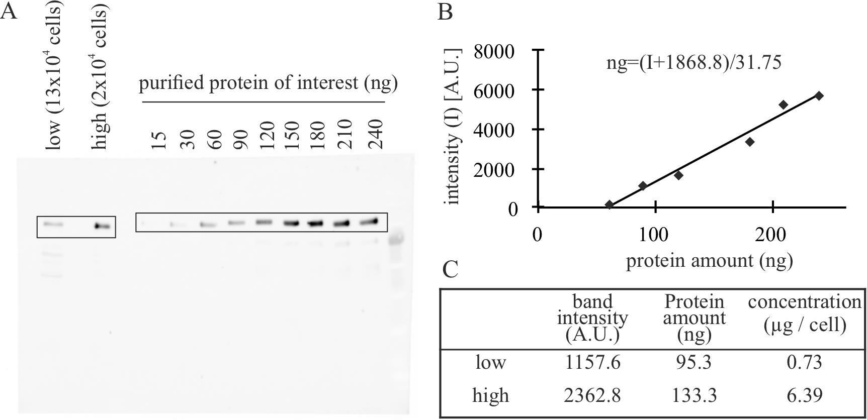
Figure 2. Example of western blot analysis to quantify the amount of protein of interest (POI) in FACS cell fractions. (A) Example of a gel for validation. Known quantities of purified POI are loaded together with lysates of known quantities of cells. Modified from Zhang et al. (2022). (B) Quantification of the bands of the gel using the gel tool analysis from ImageJ to determine the intensity of the purified POI and generate a calibration curve. (C) Combine the intensity measurements of the bands of lysates with the validation curve to obtain corrected amounts of total protein and, knowing the number of cells, the amount of protein per cell.
Extraction of total proteins from cells for western blot.
Centrifuge the cells from the sorted fractions at 0.3× g for 5 min and discard the supernatant.
Resuspend the pellet in 1 mL of lysis buffer with vigorous pipetting to disrupt the membranes.
Quantification of the amount of protein in sorted cells by western blot.
Prepare known quantities of purified POI (30, 60, 90, 120, 150, 180, 210, and 240 ng) according to the concentration calculated in A. See General note 5.
Mix the standard POI and the samples with a 4× loading buffer to a final concentration of 1× and boil them in 95 °C for 5 min. Clear the cell lysates by centrifugation at 10,000× g for 10 min and keep the supernatant on ice.
Analyze the fractions by SDS-PAGE as described before in steps A2e–A2f.
Prepare transfer buffer 1× by diluting 3 mL of transfer buffer 10× in 27 mL of H2O.
Cut Whatman papers and nitrocellulose membrane in the size of the gel and soak them in transfer buffer 1× for 15 min.
Wash the gel in H2O for 10 min.
Equilibrate the gel in transfer buffer 1× for 10 min.
Assemble the transfer unit into the transfer chamber (from down to up): 2× Whatman, nitrocellulose membrane, gel, 2× Whatman.
Remove the bubbles.
Transfer the proteins to a nitrocellulose membrane with constant 25 V for 20–45 min.
Incubate the membrane in 5% low-fat milk in PBS for 30–60 min at room temperature in a rotator.
Incubate with antibodies against your POI in the appropriate dilution overnight at 4 °C in a rotator.
Incubate with secondary antibodies linked to a fluorophore in the appropriate dilution in 3% low-fat milk in PBS for 1 h at room temperature in a rotator.
Detect the fluorescent signals using the imager (Figure 2A).
Measure the intensity in the bands using ImageJ as described before in steps A3a–A3d (Figure 1B).
Plot the intensity against the known concentrations to generate a regression curve.
Using the equation from the regression curve, calculate the protein amount for the “low” and “high” fractions of sorted cells. The intensities of the POI should be within the (linear) range of the calibration curve.
Divide the protein amount by the number of cells analyzed on the gel to obtain the number of molecules per cell.
Calculation of concentration (and use across imaging platforms)
Sample preparation. Grow the cells in the condition required in substrates suitable for imaging (i.e., chamber slides or coverslips). Follow the procedure described in step B1. See General note 6. The method is suitable for live or fixed cells. In case of fixed cells:
Remove media.
Wash the coverslips with PBS twice.
Incubate coverslips with formaldehyde solution 1:10 in PBS at room temperature for 10 min.
Wash the coverslips with PBS three times.
Add a 15 μL droplet of DAPI solution on parafilm and place the coverslips upside down. Incubate for 15 min at room temperature in darkness.
Turn the coverslips upside up.
Wash the coverslips with PBS three times.
Wash the coverslips once with H2O.
Add a 10 μL droplet of mounting media on a glass slide and place the coverslips upside down on it.
Let it dry in darkness.
Generation of calibration curve. See General note 6.
Acquire images of the cells in both negative and transfected cells with the same settings for the channel of the POI. Additionally, one can acquire additional channels to facilitate segmentations. In the examples given, we used a second channel with either DAPI (in fixed cells) or a protein that shows nuclear distribution (in live-cell imaging).
Segment the cells (or nuclei, in our case) using ImageJ (Figure 3A). In the example given, cells were segmented using the following ImageJ protocol: i) Process → Filters → Gaussian blur…, applying 2 pixels sigma (radius); ii) Process → Subtract background, applying 15 pixels of Rolling ball radius, and all other options not selected; iii) Image → Adjust → Threshold, using “Li” as threshold method. Images were then revised to find nucleus that were too close together and recognized as one to either discard them (when they overlapped) or separate into two regions of interest (when possible).
Calculate the total intensity in the channel of the POI for all cells. This value corresponds to the column “IntDen” in ImageJ result table and can be selected in Analyze → Set measurements…→ Integrated density.
Calculate the intensity values of the gates as described in Table 1 (Figure 3B).
Plot the frequencies of cells in range of the logarithm of intensity (Figure 3C).
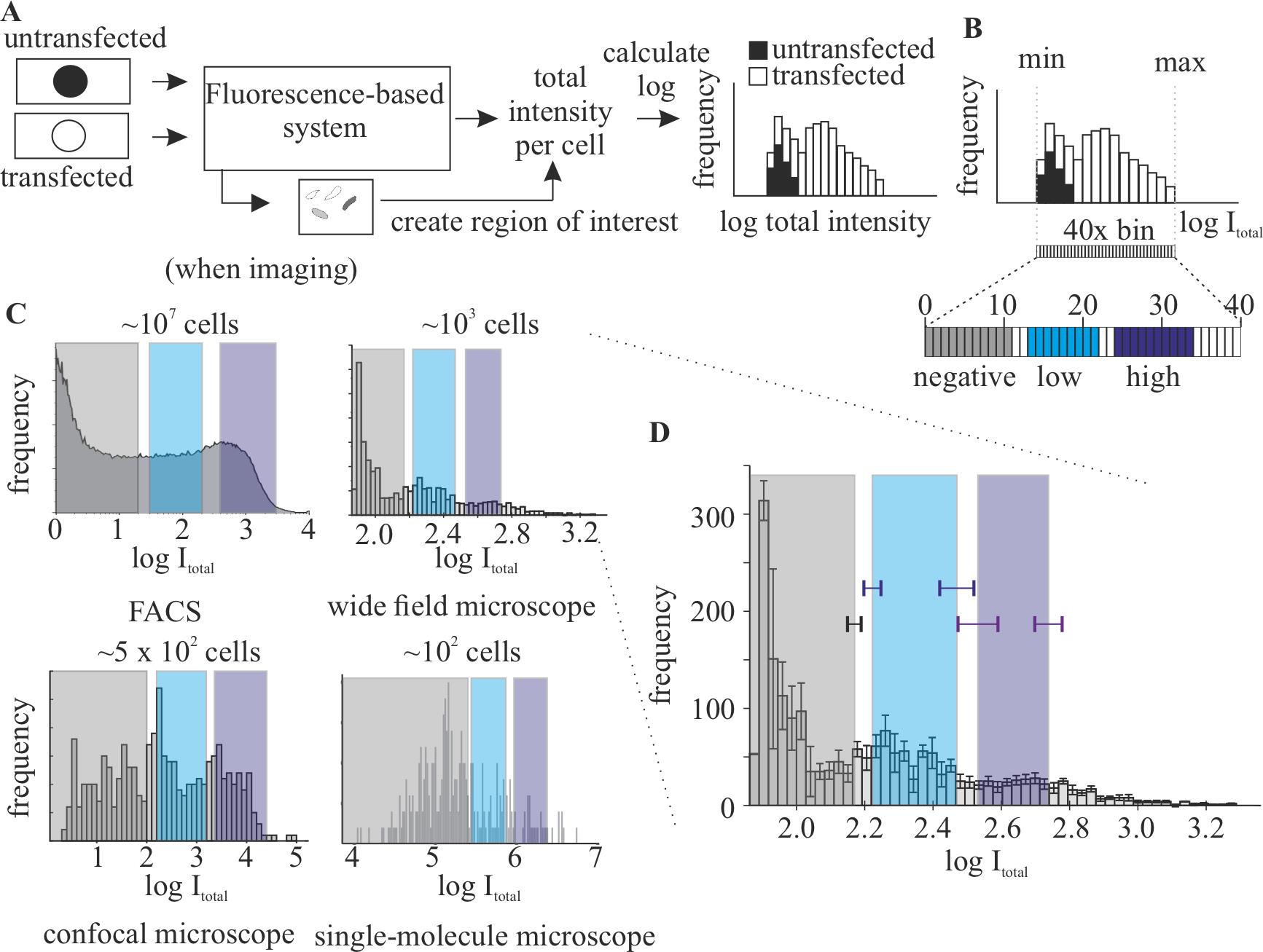
Figure 3. Generation of a calibration curve for different instruments. (A) Scheme of the minimal analysis required to generate a calibration curve in a new imaging system. (B) Calculation of the gates based on the values of intensity obtained. Bins are calculated as 1/40 of the difference between the minimal (min) and maximal (max) values observed. (C) Examples of curves for the same POI in different imaging systems: FACS (left panel), widefield (middle-left panel), confocal (right-left panel), and single-molecule microscope (right panel). Increasing the number of cells imaged leads to higher resemblance to the curve used for quantifying the protein of interest (POI) by western blot (FACS). FACS, widefield, and single molecule are modified from Zhang et al. (2022). (D) Depiction of the effects of replicates in the generation of the gates. The error bar corresponding to the three biological replicates (with n > 500 each) used to generate the widefield graph in C, including the standard deviation of the calculation of the gates using the single datasets.Check the quality of the calibration curve: all negative cells should be categorized as negative, and cells categorized as high should have a clear signal in the POI channel. See troubleshooting.
Calculation of concentration.
Acquire Z-stacks that contain the whole cellular structure where the POI is located, following the Nyquist sampling (i.e., in a confocal microscope), including the channel of the POI.
Segment the structure (additional channels can be used) and determine the intensity in the POI channel for the volume. See General note 8. In the example given, 3D segmentation was done in Volocity using the DAPI channel using the following protocol: I) Measure → Finding → Find objects; II) Measure → Processing → Dilate (iteration: 3); III) Measure → Processing → Fill holes in objects; IV) Measure → Processing → Erode (iteration: 3); V) Measure → Filtering → Exclude objects by size. The volume can be calculated from the Voxel count while the intensity is described in Sum, in the table that describes the ROIs.
Using the values for the gates of the calibration curve, classify the cells into low and high. See General note 7.
Calculate the average volume of the structure in the different categories.
The concentration of the POI for each category corresponds to the amount of protein per cell divided by the average volume of the structure for this category.
Data analysis
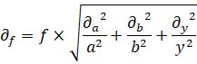
Note that, in the examples given, the protein concentration calculated for individual cells is classified in a broad category due to the selection of gates. However, the method can be as precise as it is possible to reduce the gate size and get enough cells to perform a measurable western blot. Even in this situation, there will be an error with three components: i) calculating the protein amount by western blot; ii) variability in cellular (or nuclear) volume; iii) error in the intensity measurements. Taking into account all these considerations, this method allows to assign single cells based on the POI fluorescence intensity to corresponding ranges of protein concentrations. To properly consider the mentioned errors in the final concentration number, error propagation should be taken into account at every step. In error propagation, given a function: f = a × b/y, in which the errors of the variables a, b, and y are ∂a, ∂b, and ∂c, respectively, the error of f (∂f) can be calculated as follows:
Here, you can find the sources of error and how to obtain error values:
Protein concentration for the purified protein in ng/μL (Figure 1) and in the fractions in μg/cell (Figure 2).
Intensity measurements: can be estimated as the average standard deviation of the background signal. To calculate the background signal, generate several ROIs in the same size between lines and obtain the intensities. This value corresponds to the column “IntDen” in ImageJ result table and can be selected in Analyze → Set measurements…→ Integrated density.
In replicate error: the standard deviation between the different lanes calculated (in the case of Figure 1).
Replicate error: standard deviation between technical and/or biological replicates plus the propagated error of the calculations.
Concentration of the protein in μM.
Protein concentration calculation as described above.
Volume calculation: standard deviation between cells.
In the example given in Figure 1, the background standard deviation, calculated as described in step 1a, is 15.793. Therefore, the concentrations in ng/μL for each line are 1,714.4 ± 6.8, 158.3 ± 5.5, 1,633.8 ± 4.8, and 1,601.8 ± 4.2. The final concentration number is then the average of the values, 1624.6, and the error corresponds to the standard deviation of the replicates (69.5), to which is added the propagation error of the calculations (10.8), giving the final number of 1,624.6 ± 80.3 ng/μL.
Validation of protocol
This method was validated in Zhang et al. (2022), corresponding to figures 3, supplementary figure 3, and supplementary tables S9 and S10.
For quantification, three replicates of transfected cells were sorted and analyzed with western blot to obtain the number of molecules. At least 50 cells from two biological replicates were used to calculate the volumes for the concentration for each condition.
Different calibrating curves were used in widefield microscopy (three biological replicates with approximately 500 cells per experiment) with comparable results of intensity values (Figure 3D).
To validate the use across platforms, we prepared samples as described in step B1. One-third of the cells (transfected or untransfected) were grown on coverslips and two-thirds were grown on a tissue culture dish. After 24 h, coverslips were collected, fixed with ice-cold methanol for 6 min, counterstained with DAPI, and mounted as described in steps C1d to C1i. All coverslips were imaged using a widefield microscope (Figure 4A). The DAPI channel was used for segmentation by processing in ImageJ (Gaussian blur, sigma 5 pixels; Subtract background, rolling, 20 pixels). Only nuclei with areas between 90 and 140 μm2 were considered based on our prior knowledge with C2C12 myoblasts. The calibration curve was done using the GFP intensities (Figure 4B, histogram) within the segmented nuclei. The cells grown on dishes were collected and sorted as described in steps B2 and B3, and the resulting fractions low and high were fixed with ice-cold methanol for 6 min, dried on to the coverslips by incubation at 37 °C overnight, and followed by counterstaining with DAPI and mounting as described before. These coverslips were imaged in the same conditions as the calibration (Figure 4A). The GFP intensity of the sorted cells was overlaid in the histogram (Figure 4B), resulting in segregation in the correct gates in most cases.
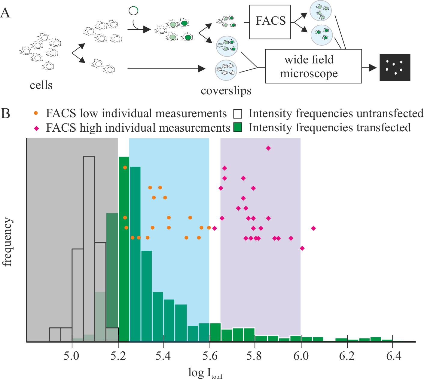
Figure 4. Validation of the reproducibility of the quantification across platforms. (A) Scheme of the validation process: cells (untransfected and transfected) were seeded in coverslips and, in parallel, a fraction of the transfected cells was sorted using fluorescence-activated cell sorting (FACS) in the categories low and high. The resulting fractions were fixed on coverslips by dehydration. All coverslips were counterstained with DAPI and imaged using a widefield microscope. DAPI was used for segmenting cell nuclei and quantifying total intensity of the GFP channel in the nucleus. (B) Non-sorted cells were used for determining the calibration curve, based on the frequencies (n untransfected: 63, n transfected: 1,539). Orange dots and magenta diamonds represent individual intensity values for the sorted low and high fraction, respectively.
General notes and troubleshooting
General notes
This material is not specifically needed for the protocol but has been used in the examples given.
Fluorescent or radioactive coupled secondary antibodies should be used for western blot to ensure linearity of the signal intensities. Enzymatic reactions (i.e., antibodies coupled to horseradish peroxidase) are not recommended.
Use tagged purified protein in cases where the protein of interest does not have suitable antibodies for western blot.
The selection of 40 bins as reference interval is meant to be versatile to generate different gate outcomes (number of categories) without changing the reference interval but can be adapted to the concrete experimental settings. Please note that the number of bins determines the range of variability that is accepted when setting gates. This step is the most susceptible to optimization when using other fluorophores and/or proteins.
The amount of protein of interest analyzed on the gel should be similar to the amount expected for the number of cells loaded. When the band corresponding to the cells is not within the calibration curve, you can modify the amounts of purified protein loaded for calibration and/or use a different number of cells.
You will need untransfected wildtype cells without a tag as negative control and transfected cells in the same conditions as described in section B for generating the calibration curve for each platform. The system is suitable for both live and fixed-cell microscopy, including immunostaining. The only requirement is that any further fluorescence, antibody, or other component should not interfere with the measurement of the intensity of the POI (i.e., overlapping of emission spectra with detection).
Each imaging instrument will require its own calibration curve. The accuracy of the measurements is highly dependent on the number of cells used for the calibration curve (Figure 3C), being ~200 cells the minimum to get reproducible results. The calibration curve can be used in the same platform, as long as the acquisition conditions (i.e., laser power, exposure time) remain constant between experiments. Please note that calibration curves should be different if single plane and volumes are used. This method should not be affected by any additional processing method (i.e., different deconvolution algorithm). If additional processing is used to determine intensities during the analysis, the images used for calibration must be treated the same way.
This section can be used to determine subcellular concentration for the POI by segmenting the subcellular structure instead of the whole cell.
Troubleshoot in calibration curves
Problem 1: Negative cells are included in the low gate.
Possible causes: (a) Dead cells with high autofluorescence have been segmented; (b) two or more cells have been segmented as one. This can be detected by plotting intensities vs. cell area; (c) bins are not accurate enough due to insufficient number of cells.
Solutions: (a) Revise the images and eliminate these cells; (b) revise the segmentation process; or (c) acquire more images from the same sample in the same conditions or merge several experiments imaged in the same conditions.
Problem 2: Transfected cells are included in the negative category.
Possible cause: Inappropriate imaging conditions (i.e., laser power or acquisition time) lead to saturation of high expressed cells.
Solution: Discard the dataset. If the dataset is extremely valuable, you can estimate the percentage of saturated cells compared to other datasets and displace the gates accordingly (note that this will add an imperfectible error!).
Acknowledgments
This work was financed by grants CA 198/10-1 project number 326470517 and CA 198/16-1 project number 425470807 to M.C.C. We thank Hui Zhang for his advice during the development of the method.
Competing interests
The authors declare no competing interests.
References
- Chiu, C. S., Kartalov, E., Unger, M., Quake, S. and Lester, H. A. (2001). Single-molecule measurements calibrate green fluorescent protein surface densities on transparent beads for use with ‘knock-in’ animals and other expression systems. J. Neurosci. Methods 105(1): 55–63.
- Dustin, M. L. (1997). Adhesive Bond Dynamics in Contacts between T Lymphocytes and Glass-supported Planar Bilayers Reconstituted with the Immunoglobulin-related Adhesion Molecule CD58. J. Biol. Chem. 272(25): 15782–15788.
- Galush, W. J., Nye, J. A. and Groves, J. T. (2008). Quantitative Fluorescence Microscopy Using Supported Lipid Bilayer Standards. Biophys. J. 95(5): 2512–2519.
- Jost, K. L., Rottach, A., Milden, M., Bertulat, B., Becker, A., Wolf, P., Sandoval, J., Petazzi, P., Huertas, D., Esteller, M., et al. (2011). Generation and Characterization of Rat and Mouse Monoclonal Antibodies Specific for MeCP2 and Their Use in X-Inactivation Studies. PLoS One 6(11): e26499.
- Kudo, S., Nomura, Y., Segawa, M., Fujita, N., Nakao, M., Schanen, C. and Tamura, M. (2003). Heterogeneity in residual function of MeCP2 carrying missense mutations in the methyl CpG binding domain. J. Med. Genet. 40(7): 487–493.
- Schindelin, J., Arganda-Carreras, I., Frise, E., Kaynig, V., Longair, M., Pietzsch, T., Preibisch, S., Rueden, C., Saalfeld, S., Schmid, B., et al. (2012). Fiji: an open-source platform for biological-image analysis. Nat. Methods 9(7): 676–682.
- Sugiyama, Y., Kawabata, I., Sobue, K. and Okabe, S. (2005). Determination of absolute protein numbers in single synapses by a GFP-based calibration technique. Nat. Methods 2(9): 677–684.
- Yaffe, D. and Saxel, O. (1977). Serial passaging and differentiation of myogenic cells isolated from dystrophic mouse muscle. Nature 270(5639): 725–727.
- Zwier, J. M., Van Rooij, G. J., Hofstraat, J. W. and Brakenhoff, G. J. (2004). Image calibration in fluorescence microscopy. J. Microsc. 216(1): 15–24.
- Zhang, H., Romero, H., Schmidt, A., Gagova, K., Qin, W., Bertulat, B., Lehmkuhl, A., Milden, M., Eck, M., Meckel, T., et al. (2022). MeCP2-induced heterochromatin organization is driven by oligomerization-based liquid–liquid phase separation and restricted by DNA methylation. Nucleus 13(1): 1–34.
Article Information
Copyright
© 2023 The Author(s); This is an open access article under the CC BY-NC license (https://creativecommons.org/licenses/by-nc/4.0/).
How to cite
Romero, H., Schmidt, A. and Cardoso, M. C. (2023). Protein Level Quantification Across Fluorescence-based Platforms. Bio-protocol 13(19): e4834. DOI: 10.21769/BioProtoc.4834.
Category
Biochemistry > Protein > Quantification
Cell Biology > Cell imaging > Fluorescence
Molecular Biology > Protein > Detection
Do you have any questions about this protocol?
Post your question to gather feedback from the community. We will also invite the authors of this article to respond.