Spatial Centrosome Proteomic Profiling of Human iPSC-derived Neural Cells

Materials and reagents

1. Human induced pluripotent stem cell lines, HMGU1 (hPSCreg: ISFi001-A) and HMGU12 (hPSCreg: ISFi002-A), obtained from the Helmholtz Center Munich iPSC Core Facility. The source of the cells is BJ fibroblasts (ATCC CRL-2522)

2. mTeSR^TM 1 culture media (basal medium and 5× supplement) (StemCell Technologies, catalog number: 05850)

3. DMEM/F-12, GlutaMAX^TM supplement (Gibco^TM, catalog number: 10565018)

4. Neurobasal medium (1×) [-] L-Glutamine (Gibco^TM, catalog number: 21103-049)

5. B-27 supplement with vitamin A (50×) (Gibco^TM, catalog number: 17504044)

6. GlutaMAX^TM supplement (100×) (Gibco^TM, catalog number: 35050061)

7. Penicillin-Streptomycin (Gibco^TM, catalog number: 15140122)

8. N2 supplement (100×) (Gibco^TM, catalog number: 17502048)

9. Non-essential amino acids (100×) (Gibco^TM, catalog number: 11140050)

10. 2-mercaptoethanol (50 mM) (Gibco^TM, catalog number: 31350010)

11. Insulin, human (10 mg/mL) (Sigma-Aldrich, catalog number: I9278-5ML)

12. Collagenase type IV (1 mg/mL) (StemCell Technologies, catalog number: 07909)

13. StemPro^TM Accutase^TM (Gibco^TM, catalog number: A1110501)

14. Geltrex Matrix, reduced growth factor (Gibco^TM, catalog number: A1413202)

15. Matrigel^® growth factor reduced (Corning^®, catalog number: 354230)

16. Laminin from Engelbreth-Holm-Swarm murine sarcoma basement membrane (Sigma-Aldrich, catalog number: L2020-1MG)

17. Poly-L-Ornithine hydrobromide (Sigma-Aldrich, catalog number: P3655-500MG)

18. Dorsomorphin (Sigma-Aldrich, catalog number: P5499-5MG)

19. SB431542 hydrate (Sigma-Aldrich, catalog number: S4317-5MG)

20. Recombinant human FGF-basic (Peprotech, catalog number: 100-18B)

21. ROCK inhibitor (Y-27632), 5 mg (StemCell Technologies, catalog number: 72304)

22. Nocodazole (Sigma-Aldrich, catalog number: M1404)

23. Dimethyl sulfoxide (DMSO), sterile-filtered (Sigma-Aldrich, catalog number: D2438)

24. Phosphate buffered saline (PBS) (10×) (Gibco^TM, catalog number: 70011044)

25. Sterile water (Braun, catalog number: 0082423E)

26. MilliQ water (Merck) or distilled water (any brand)

27. Media filter: Filtropur V25, 250 mL, 0.2 μm (Sarstedt, catalog number: 83.3940.001)

28. Media filter: Filtropur V50, 500 mL, 0.2 μm (Sarstedt, catalog number: 83.3941.001)

29. Tris-base [NH₂C(CH₂OH)₃] (Millipore, catalog number: 648310)

30. Sodium chloride (NaCl) (Sigma, catalog number: S3014)

31. Ethylenediaminetetraacetic acid tetrasodium salt (EDTA) (Sigma, catalog number: E6758)

32. Ethylene glycol-bis(2-aminoethylether)-tetraacetic acid (EGTA) (Sigma, catalog number: E4378)

33. Triton X-100 (Bio-Rad, catalog number: 1610407)

34. Sodium dodecyl sulfate (SDS) (Sigma, catalog number: L3771)

35. 2-mercaptoethanol, molecular biology grade (Sigma-Aldrich, catalog number: M3148-25ML)

36. cOmplete, Mini Protease Inhibitor Cocktail (Roche, catalog number: 11836153001)

37. Bovine serum albumin (BSA) (Sigma-Aldrich, catalog number: A2153)

38. Protein assay reagent A (Bio-Rad, catalog number: 5000113)

39. Protein assay reagent B (Bio-Rad, catalog number: 5000114)

40. Protein assay reagent S (Bio-Rad, catalog number: 5000115)

41. Dynabeads^TM protein A (Invitrogen, catalog number: 10002D)

42. Dynabeads^TM protein G (Invitrogen, catalog number: 10004D)

43. Micropipette tips (any brand)

44. 6-well cell culture dishes (Falcon^®, catalog number: 353046)

45. 10 cm cell culture dishes (Falcon^®, catalog number: 353003)

46. Cell scrapers (TPP^TM, catalog number: 99002) (Sarstedt, catalog number: 83.3951)

47. 50 mL Falcon tubes, 15 mL Falcon tubes (any brand)

48. Protein LoBind^® Tubes, 1.5 and 2 mL (Eppendorf, catalog numbers: 0030108116 and 0030108132)

49. Protein LoBind^® Tubes, 50 mL (Eppendorf, catalog number: 0030122240)

50. 5, 10, and 25 mL serological pipettes (any brand)

51. Rabbit polyclonal anti-CDK5RAP2 (Sigma-Aldrich, catalog number: 06-1398)

52. Mouse polyclonal anti-CNTROB (Abcam, catalog number: ab70448)

53. Rabbit polyclonal anti-CP110 (Abcam, catalog number: ab99338)

54. Mouse monoclonal anti-CEP170 (Invitrogen^TM, catalog number: 72-413-1/41-3200)

55. Rabbit polyclonal anti-CEP192 (Novus Biological, catalog number: NBP1-28718)

56. Rabbit polyclonal anti-CEP152 (Merck Millipore, catalog number: ABE1856)

57. Rabbit polyclonal anti-CEP63 (Merck Millipore, catalog number: 06-1292)

58. Rabbit polyclonal anti-CEP135 (Antibodies online, catalog number: ABIN2801434)

59. Rabbit polyclonal anti-POC5 (Novus Biological, catalog number: NBP1-78741)

60. Rabbit polyclonal anti-ODF2 (Abcam, catalog number: ab43840)

61. ROCK inhibitor (10 mM) (see Recipes)

62. Dorsomorphin (5 mM) (see Recipes)

63. SB431542 (10 mM) (see Recipes)

64. Poly-L-Ornithine, 10 mg/mL (see Recipes)

65. Neural maintenance medium (N3) (see Recipes)

66. Neural induction medium (N3+SMADi) (see Recipes)

67. Nocodazole (3.3 mM) (see Recipes)

68. 2 M NaCl (see Recipes)

69. 0.5 M EDTA, pH 7.5 (see Recipes)

70. 0.5 M EGTA, pH 7.6 (see Recipes)

71. 1 M Tris-HCl, pH 7.5 (see Recipes)

72. 0.5 M Tris-HCl, pH 6.8 (see Recipes)

73. 10% Triton X-100 (v/v) (see Recipes)

74. 10% SDS (w/v) (see Recipes)

75. IP/wash buffer A (see Recipes)

76. Wash buffer B (see Recipes)

77. Protein standard (BSA) (64 mg/mL) (see Recipes)

78. 1× Laemmli buffer (see Recipes)

Equipment

1. Inverted microscope (Leica, DM IL LED)

2. Neubauer improved cell counting chamber (Assistent, catalog number: 40442702)

3. Humidified cell culture incubator (any brand)

4. Brand Accu-jet pro pipette controller (Pro-lab, catalog number: 26330)

5. Microliter pipettes (Gilson^®, P1000, catalog number: 10387322; P200, catalog number: 10327282; P20, catalog number: 10082012; P2, catalog number: 10635313)

6. Ice bucket (any brand)

7. Spectrophotometer or microplate reader (any brand with 750 nm wavelength)

8. DynaMag-2 magnet (Thermo Fisher Scientific, catalog number: 12321D)

9. 1.5 mL vertical tube rotator (Stuart, catalog number: SB3)

10. Microcentrifuge with refrigeration (Thermo Fisher Scientific, catalog number: 75002446)

11. Microcentrifuge with refrigeration (Thermo Fisher Scientific, catalog number: 75004510)

12. Chemical fume hood (any brand)

13. Heating block (any brand with 95 °C capacity)

14. QExactive HF mass spectrometer (Thermo Fisher Scientific, Waltham, Massachusetts, USA)

Software

1. MaxQuant: https://www.maxquant.org/

2. Perseus: https://www.maxquant.org/perseus/

3. R Statistical Software: https://www.r-project.org/

4. Microsoft Excel: https://www.microsoft.com/de-de/microsoft-365/excel

   
   

Web resources

1. Ensembl Genome Browser: http://www.ensembl.org/index.html

2. Proteomics Identification Database (PRIDE): https://www.ebi.ac.uk/pride/

3. STRING Database: https://string-db.org/

4. Perseus documentation: http://www.coxdocs.org/doku.php?id=:perseus:start

Procedure

Table of contents and timeline:

Part I: Cell culture

A. Induced pluripotent stem cell culture media and plate preparation (0.5–1 day)

B. Induced pluripotent stem cell culture (3–5 days)

C. Induced pluripotent stem cell expansion (4–6 days × n)

D. Neural induction (40–42 days)

E. (Optional) Nocodazole treatment of the cells (4–5 h)

Part II: Protein isolation

F. Cell lysis for total protein isolation (2–4 h)

G. Assay protein concentration (0.5–1 h)

Part III: Immunoprecipitation

H. Immunoprecipitation (4–5 h)

I. Mass spectrometry (variable)

*The timeline may differ from the estimates we provide here depending on the researcher or availability of the resources.

General notes on cell culture and immunoprecipitation

1. Cell confluency is a critical element affecting proper neural induction and differentiation from iPSCs. The splitting ratios outlined in this protocol can be cell line dependent. In addition to the ratios mentioned, Table 1 outlines retrospective statistics on the range of seeding densities from different replicates of the successful differentiations using these splitting ratios. We recommend carrying out a small-scale pilot using 6-well plates in the initial instance using the splitting ratios and seeding counts outlined here as well as variations to this, such as 1:2 and 1:3, after day 10 of neural induction (Figure 1). CRITICAL: It is critical to keep the cell density above a certain level while the cells are still progenitors, i.e., still forming rosettes, to avoid their mis-direction towards other lineages.

   
   

   Table 1. Example range of cell seeding densities used across different experiments that resulted in successful neural differentiation

   *	Harvested (per cm2)	Seeded (per cm2)
   Day 0	-	350,000–550,000
   Day 10	1.2 Mio–1.7 Mio	630,000–730,000
   Day 15	690,000–1.6 Mio	300,000
   Day 21	820,000–1.4 Mio	420,000
   Day 28	480,000–850,000	190,000–250,000

   *Days since day 1 of neural induction (Mio: million)

   
   

2. It is advised to evaluate the cultures at different timepoints via immunostaining for marker proteins such as PAX6 (for neural stem cells); MAP2, CTIP2, SATB2, CUX1 (for neurons); and FOXG1 (forebrain).

   
   

   
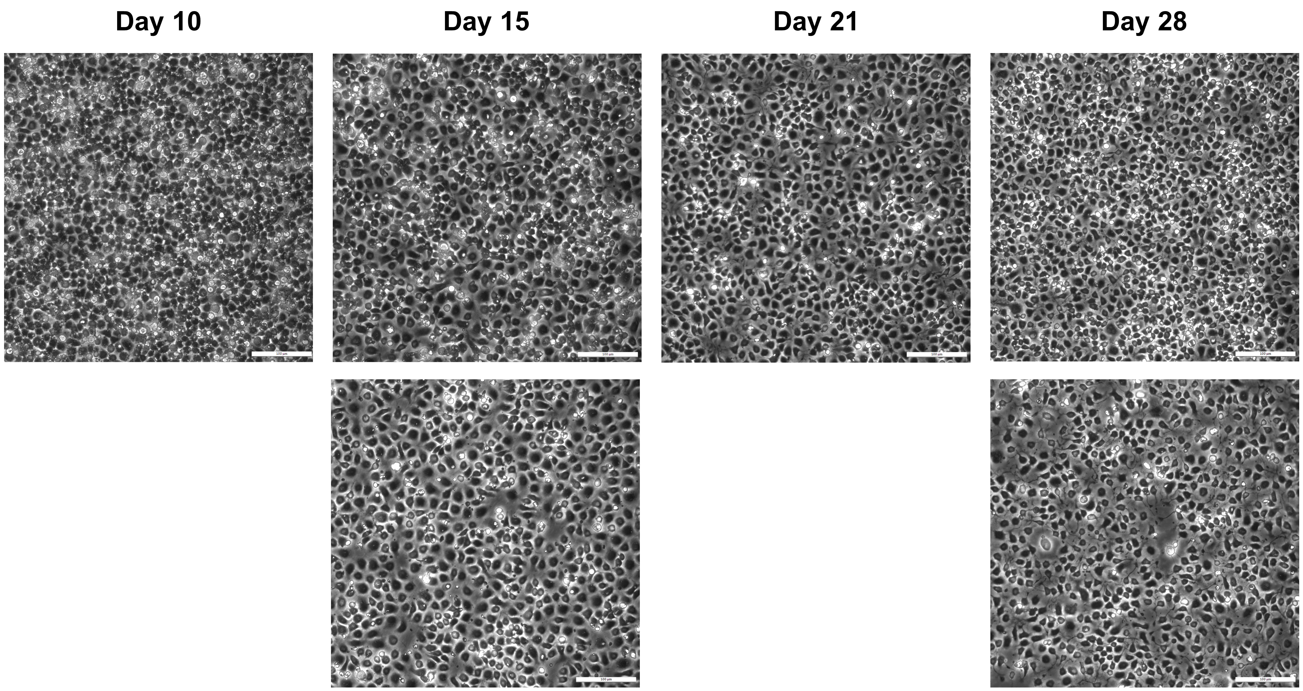
   Figure 1. Images of cells a few hours after splitting at different stages of neural differentiation. Scale bars: 200 μm.

   
   

3. Although a large amount of material is required to interrogate the full proteomic profile of the 10 baits, an advantage of this method is that the samples can be created in batches. That is, as long as all the proteomic samples across all replicates are run together on the mass spectrometer, not all of the 10 baits plus the negative controls need to be immunoprecipitated at the same time. For example, it is possible to carry out four immunoprecipitations of different baits plus a negative control in one batch, and the rest of the six immunoprecipitations plus a negative control in another batch for that cell type. The highly reproducible neural differentiation plus proteomic analysis across the four replicates makes this possible. However, if microtubule-dependent and microtubule-independent proteomic interactions are being interrogated for a particular bait (e.g., CEP120 in neural progenitors), the cells from the same batch of differentiation should be divided into nocodazole and DMSO treatments, and immunoprecipitated using the same antibody(s).

4. The protocol can easily be adapted to other cultured cell types, as well as primary cells isolated from different tissues or from different species, given the sufficient starting amount of isolated total protein for the co-immunoprecipitations can be obtained and relevant optimizations of the steps are done.

5. Unless specified otherwise, 1× PBS at room temperature is used for washing the cells.

6. It is advised to use pre-warmed media (37 °C) when splitting the cells and when changing the media daily.

   
   

Part I: Cell culture

1. Induced pluripotent stem cell culture media and plate preparation (TIMING: 0.5–1 day)

   1. Prepare the medium:

      1. When required, remove the mTeSR supplement (5×) from the freezer and thaw overnight at 2–8 °C prior to use.

      2. Aseptically add 100 mL of mTeSR supplement (5×) to 400 mL of cold (2–8 °C) mTeSR basal medium. This mixture is named mTeSR medium hereafter.

   2. Coat the plates:

      1. Thaw Geltrex on ice and dilute 1:100 in pre-cooled DMEM/F-12 medium (at 4 °C) to avoid gelling the product; mix by turning the Falcon tube upside down a few times. Add 1 mL to each well of a 6-well plate, swirl the plate to distribute the solution evenly, and incubate in a humidified cell culture incubator for at least 2 h or overnight.

      2. After incubation, remove the coating solution before seeding the cells (Optional: Wash the wells once with 1–2 mL of sterile 1× PBS). PAUSE POINT: If not using straight away, add 2 mL of 1× PBS per coated well, wrap the plate with parafilm, and store at 2–8 °C for up to one week.

         
         

2. Induced pluripotent stem cell culture (TIMING: 3–5 days)

   Note: Before thawing the cells, have the Geltrex-coated plate(s), medium, ROCK inhibitor ready, and warm the water bath to 37 °C.

   1. Prepare mTeSR medium supplemented with 10 μM ROCK inhibitor (1:1,000 dilution of 10 mM stock solution) sufficient for thawing and seeding the iPSCs as described below (hereafter referred to as mTeSR+ROCKi).

   2. Pre-warm 3–4 mL of mTeSR+ROCKi to 37 °C in a 15 mL Falcon.

   3. Rapidly thaw a vial of viable iPSCs frozen at a density of 2 × 10⁵–1 × 10⁶ (or one well of a 6-well plate) by placing the cryovial in a water bath at 37 °C for 1–2 min (until a tiny ice particle remains).

   4. Using a 1 mL sterile pipette, transfer the cells into the pre-warmed 15 mL Falcon tube containing mTeSR+ROCKi. TIP: Disinfect the cryovial with 70% ethanol before opening.

   5. Centrifuge at 300× g for 4 min at room temperature and remove the supernatant.

   6. Resuspend the cells in 1.5–2 mL of mTeSR+ROCKi. Remove the Geltrex/PBS from the Geltrex-coated plate and add the cell suspension mixture to a single well of the 6-well plate (or up to three wells, with at least 1.5 mL final media in each).

   7. Rock the plate side-to-side in both directions to evenly distribute cells in the well and incubate at 37 °C, 5% CO₂.

   8. The next day, remove the medium, wash the cells once with 1× PBS, add 1.5 mL of fresh mTeSR without ROCK inhibitor per well, and incubate at 37 °C, 5% CO₂.

   9. Replace the medium with 1.5 mL of fresh mTeSR every day until the cells are 80% confluent. Optional: When the cells are more than ~70% confluent, 2 mL of medium can be used instead.

   10. It is good practice to observe iPSC lines under a phase contrast microscope daily to check for iPSC-like morphology, presence of differentiated cells, and confluency (Figure 2).

       
       

       
       Figure 2. Induced pluripotent stem cells (iPSCs) at different growth phases. A) A few days after splitting. Cells might look larger, with loose cell-to-cell contacts. B) Semi-confluent stage. Center of the colonies has round cells with tight contacts, while the growing edges contain looser cells. C) With high confluency, most of the iPSCs become round and compact with tight cell-to-cell contacts. Scale bars: 200 μm.

       
       

3. Induced pluripotent stem cell expansion (TIMING: 4–6 days × n)

   Notes:

   1. Here, we describe splitting the cells from one well of a 6-well plate to six wells (1:6 splitting ratio). Size of the plates, volumes, and the ratio can be up- or down-scaled.

   2. Have a 6-well plate coated with Geltrex ready on the day of splitting.

   3. We describe here the passaging of the iPSCs using a combination of enzymatic and mechanical approaches. First, the wells are treated with Collagenase IV to soften the basement membrane, and then the cell clumps are collected using a cell scraper and further dissociated mechanically.

   4. Dilute the Collagenase IV 1/4 in 1× PBS and keep aliquots in Falcons at -20 °C. Once thawed, working solution can be kept at 2–8 °C for a few weeks and should not be re-frozen.

      
      

   1. For splitting the cells, pre-warm at least 1 mL of Collagenase and 9 mL of mTeSR to 37 °C. Volumes can be slightly increased to account for pipetting loss.

   2. Aspirate the media from the well and add 2 mL of sterile 1× PBS. Swirl the plate a few times and remove the PBS.

   3. Add 1 mL of Collagenase (1/4 in 1× PBS) to the well, distribute equally by swirling, and incubate the plate at 37 °C for 5 min (no more than 8 min, as the cells should not detach at this stage yet).

   4. Aspirate Collagenase and add 1 mL of 1× PBS or mTeSR.

   5. Scratch the well first with a 200 μL pipette tip at different directions to break cell colonies. Then, use a cell scraper to detach the cells from the plate completely.

   6. Using a 1 mL pipette (or a serological pipette, depending on the number of wells) transfer the cells into a 15 mL Falcon and centrifuge at 300× g for 4 min at room temperature. Alternatively, keep the falcon at room temperature for 5-8 minutes for the cell clumps to precipitate to the bottom of the Falcon tube.

   7. While cells are spinning, add 1 mL of mTeSR (pre-warmed to 37 °C) to each of the six Geltrex-coated wells.

   8. Once cells have finished spinning, aspirate the supernatant and resuspend the cell pellet in 3 mL of fresh mTeSR, by pipetting the media up and down quickly 5–8 times. CRITICAL: Make sure to have neither single cells nor very large cell clumps. Clumps of 10–30 cells can be ideal. If the cells are too much dissociated by mistake, add ROCK inhibitor (10 μM final) for one day to help their survival. If the clumps are too large, iPSCs tend to differentiate in the middle of the colonies before the plate becomes confluent. To avoid large clumps, cells can be pipetted up and down additionally a few times before seeding to break them up further.

   9. Add 0.5 mL of resuspended cell mixture to each of the six wells. Rock the plate side to side in both directions a few times and incubate the cells at 37 °C, 5% CO₂. TIP: Avoid swirling the plate, as it will cause the cells to accumulate in the center of the well and start differentiating after a few days due to high density.

   10. The next day, replace the media with 1.5 mL of fresh mTeSR, and repeat this step every day. Optional: When the cells are more than ~70% confluent, 2 mL of medium can be used instead.

   11. Once at 80% confluency, split the cells again.

   12. Continue expansion until having enough cells for neural induction.

       
       

4. Neural induction (TIMING: 40–42 days)

   Note: Here, we describe a protocol for generating 60–100 × 10 cm dishes with neurons at day 40 of differentiation (Figure 3). This can account for 11 immunoprecipitations (IPs) for each of DMSO and nocodazole treatments (22 IPs in total, including negative controls) (Figure 4). Number of plates and IPs can be up- or down-scaled. For each 10 cm dish on day 0, grow 3–5 wells of 80% confluent iPSCs (Table 1). Along the differentiation, adjust the number of plates to proceed in each splitting according to the final number of plates desired. For neurons, calculate some additional plates to account for potential partial detachment of the cells, especially after day 35 of the differentiation.

   
   

   
   Figure 3. Schematic representation of expansion and differentiation of induced pluripotent stem cells (iPSCs) towards neurons for co-immunoprecipitation of centrosome proteins with their interactors

   
   

   
   Figure 4. Statistics (A) on the number of plates with day 40 neurons vs. total protein (milligrams) obtained in different sparse (B) or normal density (C) batches. Scale bars: 200 μm.

   
   

   1. Dilute Matrigel 1:300 from an 8–12 mg/mL stock in DMEM/F-12 medium and add 4–4.5 mL per each of the two 10 cm dishes. Leave at 37 °C, 5% CO₂ from at least 4 h to overnight.

      1. CRITICAL: Do not let the coating dry on any part of the plate, as this alters the attachment of the cells and success of the induction. If part of the plate dries out, this might generate a heterogenous population of cells, which is impossible to sort out later. Therefore, adjust the coating volume carefully.

      2. Before seeding the cells, remove the coating solution (Optional: Wash with 3 mL of 1× PBS).

      3. PAUSE POINT: If the coated plates will not be used immediately, store at 4 °C after adding 6 mL of fresh 1× PBS up to two weeks.

   2. Pre-warm Accutase and mTeSR medium to 37 °C.

   3. Remove the media from 6-well plates containing iPSCs and wash once with 1× PBS.

   4. Add 0.5–0.7 mL Accutase to 7–10 wells containing iPSCs (leave one well for re-splitting as per section C1) and incubate at 37 °C, 5% CO₂ for 5 min (no longer than 8 min) (Optional: Swirl the plate once in the middle of the incubation). At the end of the incubation, cells should be suspended in solution mostly in single cell form.

   5. After 5 min, add 1 mL of mTeSR or 1× PBS to each well containing Accutase and carefully collect and pool all the cells in a Falcon tube. Centrifuge at 300× g for 4 min at room temperature.

   6. Remove the supernatant, being careful of the cell pellet. Resuspend the cells with 6 mL of mTeSR at 37 °C supplemented with 10 μM ROCK inhibitor (mTeSR+ROCKi).

   7. Add 3 mL of cells to each of the 10 cm dishes pre-filled with mTeSR+ROCKi, to have a final volume of 10 mL.

      1. From our experience, 3–4 confluent wells of a 6-well plate suffice for seeding a 10 cm dish.

      2. Alternatively, count cells and seed 350,000–550,000 cells per cm² of the 10 cm dish (Table 1) and adjust the final volume to 10 mL.

      3. CRITICAL: It is important to have a dense cell layer of iPSCs on day 1 for proper neuroectoderm induction (Figure 5, Day1). With lower densities, the cells might assume neural crest-like or other lineages (Liu et al., 2015; Hindley et al., 2016).

         
         

         
         Figure 5. Example images from different stages of successful differentiations. Cells were split on days 10, 15, 21, and 28. Days 11, 16, 22, and 29 represent the days after splitting. Day 15 and 40 are the timepoints used for the proteomic analysis in O’Neill et al. (2022). Scale bars: 200 μm.

         
         

   8. After seeding, rock the plates from side to side in both directions a few times to homogenously distribute the cells after placing into the incubator (avoid swirling) and keep at 37 °C, 5% CO₂ overnight.

      The next day, if cells completely cover the entire plate (Figure 5, Day 1), begin neural induction. If not, replace with fresh mTeSR and incubate for another day. Do not keep the seeded cells more than two days before the induction.

   9. The next day, remove the media, wash the cells once with 1× PBS, and replace with 10 mL of neural induction medium (N3+SMADi). This represents day 1 of neural induction.

   10. Neural induction medium (N3+SMADi) is changed every day until day 10 of differentiation when a uniform neuroepithelial sheet should have formed.

   11. On/before day 10, have the poly-L-ornithine/Laminin-coated plates ready, as follows:

       1. Thaw a 10 mg/mL aliquot of poly-L-ornithine (PO). TIP: Keep the PO aliquot at 4 °C after thawing.

       2. Coat four 10 cm dishes with poly-L-ornithine diluted 1:500 in sterile water. Incubate at 37 °C, 5% CO₂ for at least 4 h. To be on the safe side, add at least 4.5 mL of coating solution per 10 cm dish to prevent partial drying out.

       3. Following coating, remove the PO solution (optional: wash the plates once with 1× PBS) and coat the plates with Laminin diluted 1:200 in 1× PBS. Incubate at 37 °C, 5% CO₂ for at least 4 h (or overnight). CRITICAL: Do not let the Laminin coating dry on any part of the plate, as this influences the density of attached cells, which is critical for the neural differentiation.

       4. The same PO+Laminin coating procedure can be applied to sterile glass coverslips in 24-well plates to seed the cells for immunostaining.

       5. PAUSE POINT: If the PO+Laminin-coated plates will not be used immediately, they can be stored after adding 6 mL of 1× PBS and sealed with parafilm at 2–8 °C for up to four weeks. Nonetheless, we recommend coating freshly before each splitting.

   12. At day 10 of neural induction, split the cells 1:3. The exact splitting ratio can vary across cell lines but should be aimed at reaching 100% confluency on day 15 (Table 1, Figure 5).

       1. Wash the cells with 1× PBS after removing the media, add 2 mL of Accutase per 10 cm dish, and incubate at 37 °C, 5% CO₂ for 5 min.

       2. Add 3 mL of neural induction medium (N3+SMADi) or 1× PBS to each plate, mechanically dissociate cells with a rubber (TPE) cell scraper, and then collect in a 50 mL Falcon.

       3. Spin at 300× g for 4 min.

       4. Remove the supernatant being careful of the cell pellet and re-suspend the cells with 18 mL of N3+SMADi supplemented with ROCK inhibitor (10 μM) (N3+SMADi+ROCKi) (assuming the cells were collected from 2 × 10 cm dishes).

       5. Dispense cells according to a 1:3 ratio (in this case, 3 mL of cell suspension per 10 cm dish pre-filled with 5 mL of N3+SMADi+ROCKi) and incubate at 37 °C, 5% CO₂. Optional: Count cells and seed according to the ranges provided on Table 1.

   13. The next day (day 11), replace media with N3 medium without ROCK inhibitor. Replace the media again on day 12.

       If the growing rate of cells do not forecast reaching to 100% confluency at day 15, supplement the media with 4 ng/ml FGF (1:2,500 dilution of 10 µg/ml stock) on day 11 or day 12, and keep with this medium for only one day. Avoid high doses or extended periods of culture with FGF, as it might caudalize the cells.

   14. From day 12 on, replace the medium with fresh N3 every other day (unless FGF is added; if so, adjust the media changing days accordingly).

   15. On day 15, cells should be 100% confluent with the appearance of rosettes (Figure 5).

       1. TIP: If the rosettes are not readily visible, try to observe them while washing the cells with PBS or after changing the media.

       2. If the cells were also seeded on the coverslips, fix them with PFA (to stain for cell identity markers, such as PAX6) or methanol (to stain for most centrosome proteins).

   16. On/before day 15, have the poly-L-ornithine/Laminin-coated plates ready and split the cells as described for day 10 from section D12 onwards.

   17. From this stage on, replace the media every second day (8 mL of N3 per 10 cm dish). Always replace the media the day after splitting the cells, preferably after washing the cells once with 1× PBS.

   18. Split the cells also on days 21 and 27/28 (for approximate cell counts, refer to Table 1) and proceed with media changes until day 40 (Figure 3). TIP: From approximately day 35 on, be extra careful when changing the media, as the cells tend to detach locally or as an entire sheet from the plate. To avoid this, either add the medium very slowly using a 25 mL pipette dropwise or change only half of the media, but daily.

   19. Observe the morphology of the cells along the differentiation to see if they assume morphologies typical of each stage (Figures 5 and 6).

       
       

       
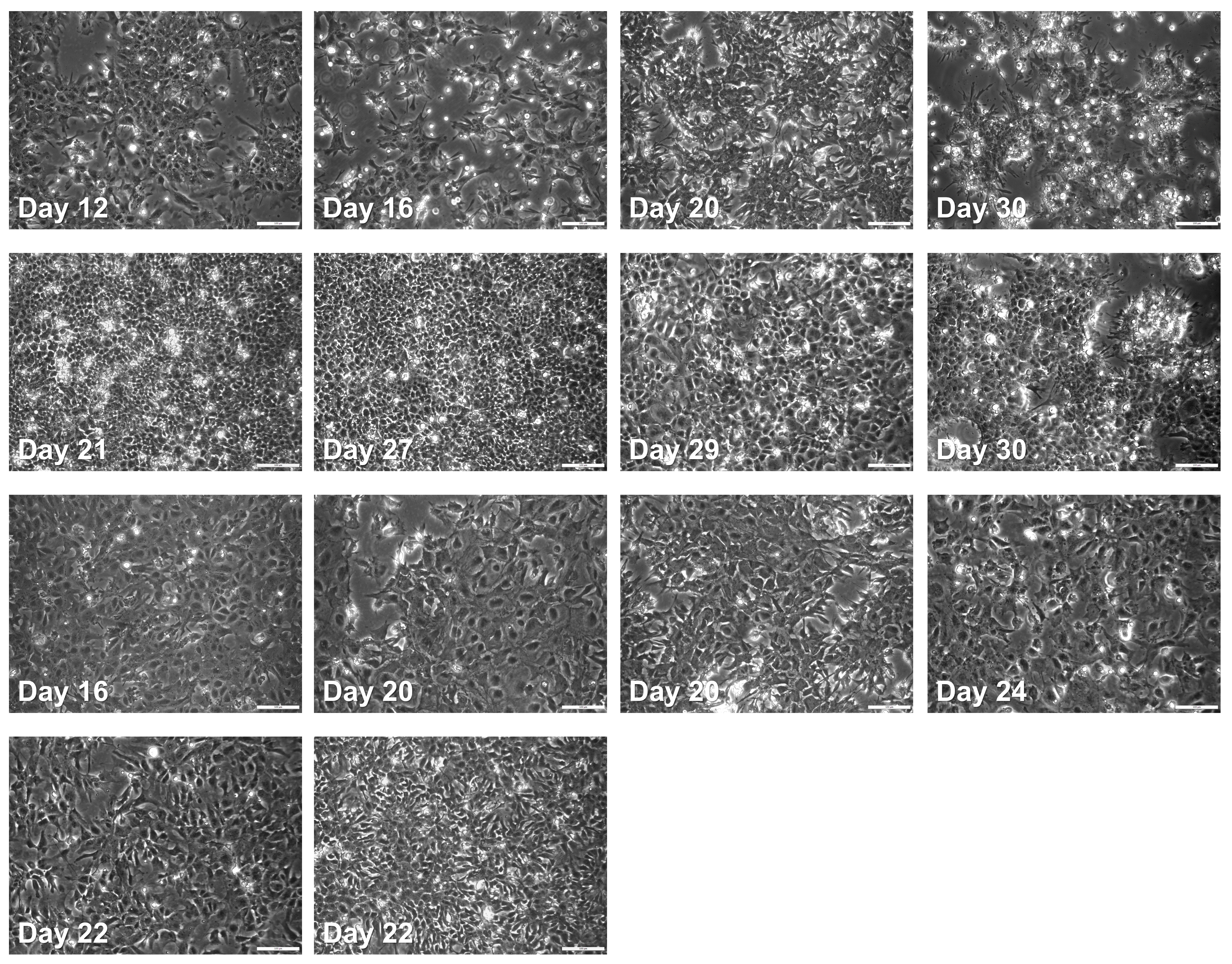
       Figure 6. Example images from failed differentiations. Cells might assume cobblestone or spiny/fibroblast-like morphology, have large and/or darker nuclei, or enlarged cytoplasm. Cultures should be monitored frequently (e.g., after each media change) to watch out for such aberrant morphologies, which might signal potential failure of the differentiation. Scale bars: 200 μm.

       
       

5. (Optional) Nocodazole treatment of the cells (TIMING: 4–5 h)

   Notes:

   1. Nocodazole is a drug that blocks polymerization of the microtubules and can be used to assess microtubule-independent centrosome interactions of the proteins. To this end, nocodazole and DMSO (solvent, as control) are added to their respective culture plates 4 h before harvesting the cells for protein isolation and immunoprecipitation (Figure 7).

      
      

      
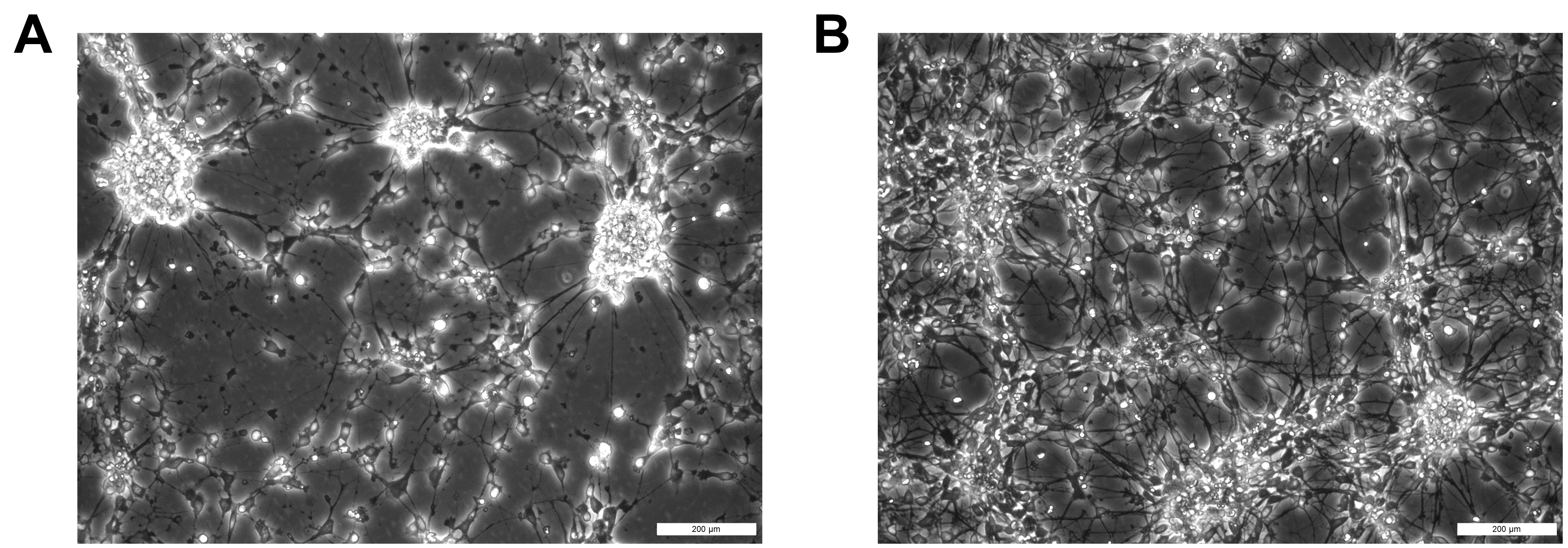
      Figure 7. Day 40 neurons after 4 h of nocodazole treatment. A) Nocodazole-treated cells B) DMSO-treated control cells. Scale bars: 200 μm.

      
      

   2. Because nocodazole increases cell death and reduces protein yield, plates can be divided into nocodazole and DMSO treatments with approximately 60:40 ratio to account for this loss.

   3. For microtubule depolymerization, alternative agents such as vinorelbine, vincristine, colchicine (Bates and Eastman, 2017), or cold exposure (Li and Moore, 2020) can also be considered and tested to see if they result in reduced cell death.

      
      

   1. Add nocodazole (3.3 mM stock concentration, dissolved in DMSO) to a final concentration of 3.3 μM to the N3 medium (1:1,000). Swirl plate to distribute it evenly.

   2. As a control, DMSO is added to its respective plates using the same ratio added to the nocodazole plates (i.e., 1:1,000).

   3. Incubate the plates at 37 °C, 5% CO₂ for 4 h, confirm the de-polymerization under the microscope, and begin collecting the cells for lysis and protein isolation.

      
      

Part II. Protein isolation

6. Cell lysis for total protein isolation (TIMING: 2–4 h)

   Notes:

   1. On the day of immunoprecipitation (IP), freshly make up IP/wash buffer A and wash buffer B and store on ice for the duration of the procedure.

   2. Cool centrifuge for spinning 50 mL Falcons to 4 °C.

   3. Pre-cool 1× PBS to 4 °C and keep in the ice bucket (in case of nocodazole treatment).

      
      

1. Obtain plates from incubator and aspirate the media. Wash cells with 3 mL of 1× PBS per plate. Aspirate PBS and add 3 mL of fresh 1× PBS.

   1. TIP: If handling a lot of plates, you can split them to batches, keeping the rest in the incubator.

   2. For nocodazole-treated plates, wash with ice-cold PBS, keep plates on ice in bucket while scraping, and process only a couple of plates at a time acting quickly to impede repolymerization of microtubules. TIP: To keep the conditions as similar as possible, DMSO-treated plates can be treated the same way.

2. Using a cell scraper, scrape the cells off the plate, tilting the plate sideways and pushing all the cells into the PBS. Keep the plate tilted and, using a 10 mL pipette, transfer cells in PBS to a 50 mL Falcon placed on ice.

3. Continue to scrape cells and transfer to 50 mL Falcon tube(s), pooling the cells within their respective treatments.

4. Once all plates are scraped (or the 50 mL Falcon is filled), spin at 300× g for 5 min at 4 °C to pellet cells.

   1. Aspirate off the PBS (ensure the pellet is not removed).

   2. PAUSE POINT: If cell lysis will not be done on the same day, cell pellets can be snap-frozen in liquid nitrogen and kept at -80 °C. If this is the case, add the IP/wash buffer A directly on the frozen pellet without thawing it on the day of lysis.

5. Assess the volume of the pellet in milliliters and add double that volume of IP/wash buffer A.

6. Incubate on ice for 30 min.

   It is important not to dilute the sample too much, as this will affect the protein concentration and subsequent downstream steps. For example, 5 mg of total lysate in 1 mL will be used for immunoprecipitation; therefore, the concentration should not be lower than this.

7. During the cell lysis, cool a micro-centrifuge capable of spinning 1.5 mL tubes at 18,000× g to 4 °C.

8. After the 30 min incubation, once the cells are lysed, distribute lysate into 1.5 or 2 mL protein low bind tubes and spin at 18,000× g for 10 min at 4 °C to pellet the cellular debris.

   During this time, set up the protein standards for the standard curve as described below.

9. After the 10 min centrifugation and the cellular debris is pelleted, carefully remove the clear supernatant from the 1.5 mL tubes and pool into a (Optional: protein low bind) 15 mL Falcon (CRITICAL: do not mix different samples), mix well, and proceed with the next step. TIP: It can be practical to calculate the total volume while pooling the lysates for a more accurate estimation of total protein later.

   PAUSE POINT: If the cell lysates will not be used immediately, they can be kept at -80 °C.

   
   

7. Assay protein concentration (TIMING: 0.5–1 h)

   Notes:

   1. Prepare the dilutions and protein standards on ice.

   2. Adding the reagents to the microplate and subsequent steps can be done at room temperature.

      
      

   1. To set up the protein standards, add 20 μL of IP/wash buffer A to six individual tubes (labeled as 8, 4, 2, 1, 0.5, 0.25). Add 20 μL of the 16 mg/mL BSA protein standard (see Recipes) to the first tube (8 mg/mL), performing a 1:2 dilution series with the remaining tubes, down to 0.25 mg/mL.

      Example: mix [20 μL of buffer A + 20 μL of standard], transfer 20 μL of this mixture to the next tube that already contains 20 μL of buffer A, mix well, transfer 20 μL of this mixture to the next tube, and so on.

   2. In a fresh tube, make a master mix with a 49:1 ratio of Reagent A and Reagent S (A+S) of the Bio-Rad Protein Assay:

      Calculate two replicate wells per four standards (2 mg/mL, 1 mg/mL, 0.5 mg/mL, and 0.25 mg/mL), one for control, two replicates per sample to be measured, and two extras (Figure 8). Example:

      
      

      A+S mix = [11 + (2 × N_samples)] × (24.5 μL Reagent A + 0.5 μL Reagent S)

      
      

      
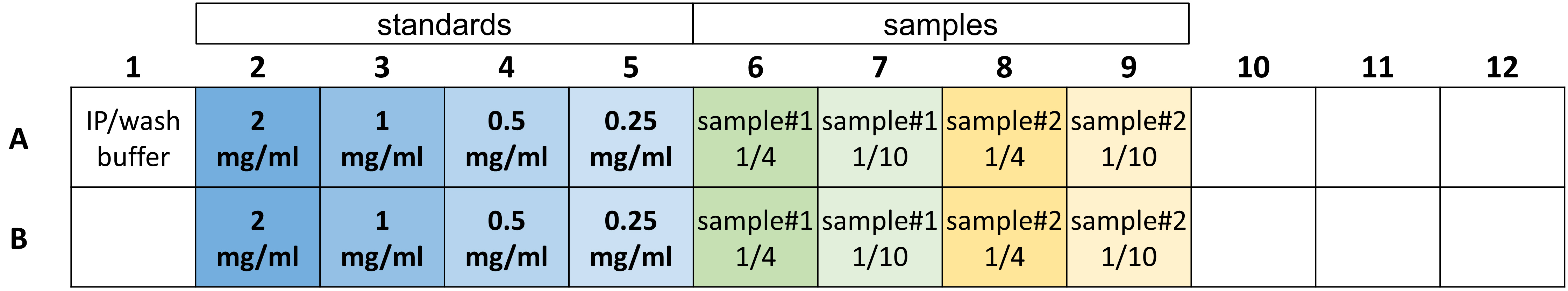
      Figure 8. Example layout of a microplate section with protein standards and diluted samples for determination of protein concentration with DC Protein Assay

      
      

   3. Add 25 μL of the A+S mix to the wells of the protein reader plate.

   4. Add 5 μL of each protein standard to two corresponding wells each, as well as the 5 μL of IP/wash buffer-only control to its respective well (Figure 8).

   5. Add 5 μL of the cell lysate per sample to their respective wells containing the A+S mix.

      If the protein concentration is too high, the measurement will fall above the linear range. In this case, two different dilutions of the samples can be used for measurement, e.g., 1/4 and 1/10, or else, to ensure accurate determination of concentration. Try to make sure at least one of your sample dilutions fall within the range of 2–0.25 mg/mL.

   6. Aliquot 200 μL of Reagent B to each well to be measured, going from the lowest-to-highest protein concentration wells, and incubate at room temperature for 10–15 min.

   7. Measure the absorbance of the samples at 750 nm within one hour and use the protein standard measurements to produce a standard curve using linear regression (y = mx + n) where y is absorbance and x is protein concentration. Then, calculate the amount of protein within your sample(s) of interest based on its absorbance using this formula.

      1. TIP: It is not recommended to exceed 2 mg/mL for the standards, as the linear range can be lost for higher values than this. Calculate the R² value of the fitted line to check its linearity.

      2. PAUSE POINT: If the cell lysates will not be used immediately, they can be kept at -80 °C.

         
         

   Part III: Immunoprecipitation

   8. Immunoprecipitation (TIMING: 4–5 h)

      Note: At least four replicate immunoprecipitations performed using different biological replicates are recommended for each bait of interest.

      1. Calculate how many immunoprecipitations can be performed with the total lysate obtained from cells (Figure 4).

         1. Each immunoprecipitation for mass spectrometry requires 4–5 mg of starting total protein, while samples for assessing the immunoprecipitation by Western blot can be as little as 500 μg.

         2. Each immunoprecipitation is performed in 1 mL of volume.

      2. Dilute the protein lysate to 5 mg/mL in IP/wash buffer A and aliquot 1 mL of lysate into each respective protein low bind tube for immunoprecipitation. Keep the samples on ice.

         1. For every set of immunoprecipitations, one of the samples should be reserved for no-antibody control.

         2. As an alternative to the no-antibody control, it is encouraged to use isotype-specific control antibody(s) as negative control that matches the class and type of the primary antibodies used in the experiment.

      3. For each immunoprecipitation, add 2 μg of the desired antibody to 1 mL of lysate at 5 mg/mL. For the negative control, add no antibody to the tube or add the isotype control. CRITICAL: From this point on, be very careful about cross-contamination of the samples. Never use the same tips for different samples during washes and avoid splashes across the tubes, as mass spectrometry has a very-high detection sensitivity.

      4. Incubate tubes on an end-to-end rotator in a 4 °C cold room for 1 h. Fifteen minutes before the end of this incubation, prepare the Protein A and Protein G Dynabeads solution:

         1. Mix 10 μL of Protein A and 10 μL of Protein G per immunoprecipitation (including the negative control) in a 1.5 mL tube. Example:

            A+G mix = (1 + N_IPs) × (10 μL Protein A + 10 μL Protein G)

         2. Place tube on a magnetic strip and remove the liquid without disturbing the beads with the pipette tip.

         3. Resuspend the beads with IP/wash buffer A using the same volume aspirated from the tube, place the tube on the magnetic strip, and remove the liquid.

         4. Repeat this wash two more times and finally re-suspend the beads with IP/wash Buffer A using the original volume.

      5. After 1 h incubation of the lysate with the antibodies, add 20 μL of Protein A+G mix to each IP tube as well as to the negative control. Incubate on the rotator for an additional 2 h at 4 °C.

      6. After this incubation period, place all the IP tubes on the magnetic strip. Remove the wash buffer, leaving the beads coupled to the antibodies and protein attached to the wall of the tube. Add 1 mL of IP/wash buffer A.

         CRITICAL: Use a clean tip for each sample to remove the supernatant.

         CRITICAL: Work very quickly or in batches to avoid drying of the beads if there are too many samples.

      7. Incubate the samples on a rotator at 4 °C for 15 min and repeat the above step two more times (each with a 15 min incubation).

      8. During this process, pre-heat a heating block to 95 °C.

      9. Under a chemical hood, mix 1× Laemmli buffer and 2-mercaptoethanol in a 39:1 ratio (e.g., 975 μL of 1× Laemmli buffer + 25 μL of 2-mercaptoethanol). Approximately 30–40 μL is required per IP.

      10. After the third wash, place the samples on the magnetic strip and remove the wash buffer. Add 1 mL of wash buffer B to each sample before incubating on a rotator at 4 °C for a couple of minutes. Repeat this step once again.

      11. After these washes, place the samples on the magnetic strip and remove the wash buffer. TIP: 10/20 μL tip can be used following the 1,000 μL tip to remove the supernatant as much as possible. Place the tubes with the beads immediately on ice and transfer to a fume hood.

      12. Add 30–40 μL of fresh Laemmli buffer containing 2-mercaptoethanol to each sample and ensure the beads are well re-suspended. The volume can be decided on a case-by-case basis, but it is important to keep it consistent across different samples and batches.

      13. Incubate the tubes for 10 min at 95 °C. After this time, place the tubes on the magnetic strip in the fume hood and transfer the supernatant (Laemmli buffer now also containing the immunoprecipitated protein of interest and its interactors) to a new protein low bind tube without disturbing the beads.

      14. Store samples at -80 °C until all immunoprecipitations are completed. CRITICAL: Run all samples together on the mass spectrometer, as run-to-run variations are common even if the same samples are re-analyzed at a different timepoint.

          
          

   9. Mass spectrometry

      1. LC-MS/MS analysis of the eluates from the co-immunoprecipitations was performed on a QExactive HF mass spectrometer, as described in O’Neill et al. (2022).

      2. Proceed to the MaxQuant section once the .RAW files from mass spectrometry are available.

Data analysis

Table of contents and timeline:

Part I: MaxQuant analysis

A. Processing the mass spectrometry. RAW files using MaxQuant (3–10 days)

Part II: Perseus analysis

B. Pre-processing, annotation, and quality control (0.5–2 days)

C. Statistical analysis (2–7 days)

Part III: Further analysis

D. Combine and summarize the data (0.5 day)

E. Further analysis suggestions (variable)

*The timeline may differ from the estimates we provide here depending on the researcher or availability of the resources.

General notes on data analysis

The data analysis section contains the following main parts (Figure 9):

1. Processing the mass spectrometry .RAW files to generate intensities (MaxQuant)

2. Pre-processing, annotation, and quality control (Perseus & R statistical software)

   1. Importing the MaxQuant output into Perseus

   2. Annotating the samples

   3. Quality filtering

   4. [Optional: Adding pathway annotations (e.g., KEGG pathway, GO terms)]

   5. Cluster analysis for quality control (Perseus & R statistical software)

3. Statistical analysis (Perseus & Excel)

   1. t-test (volcano plot)

   2. Ranking the proteins for statistical significance

4. Combining and summarizing the data (R statistical software)

5. Network analyses

   Intermediate files generated along this protocol and R scripts are provided in the Supplementary information.

   
   

   
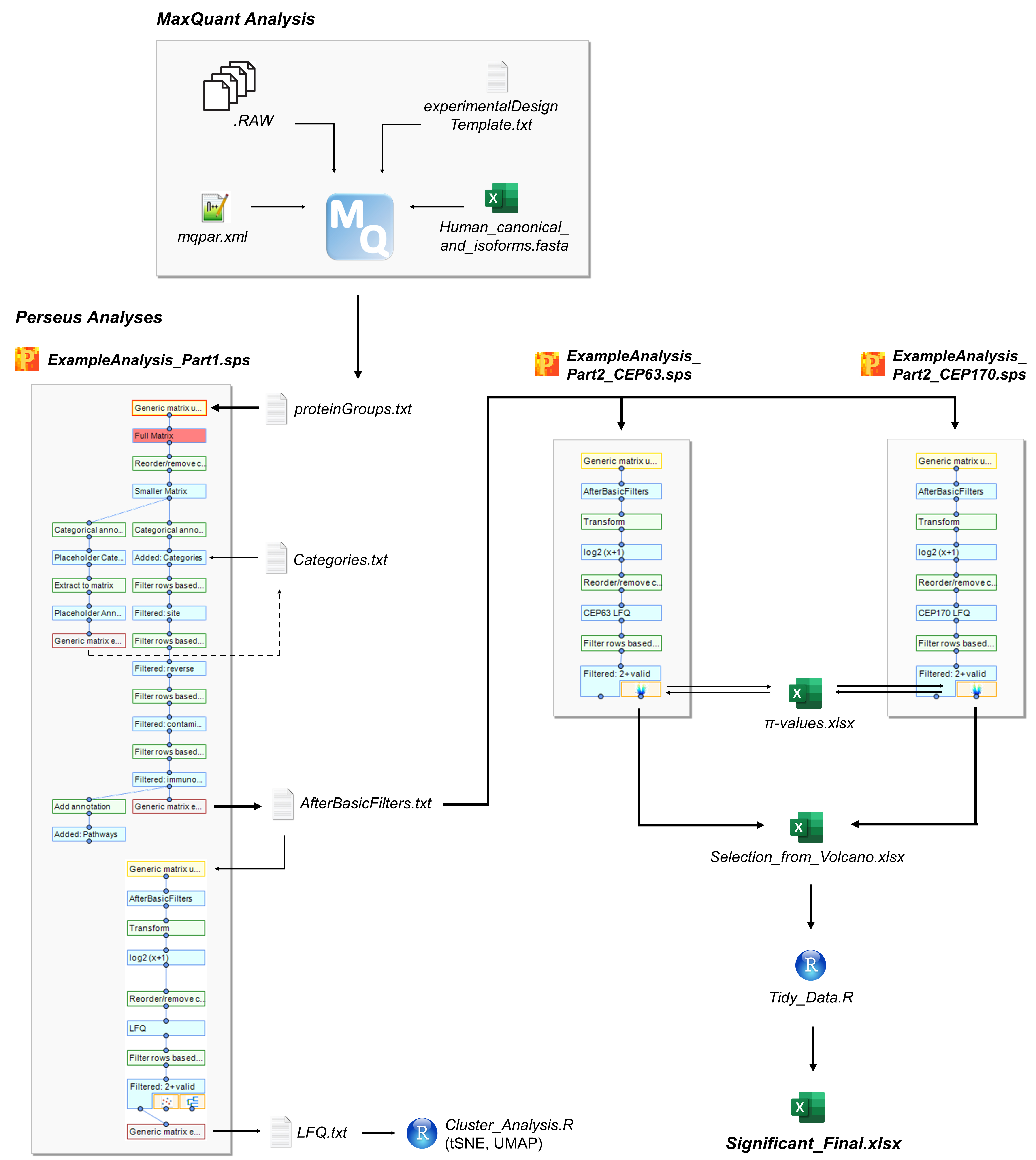
   Figure 9. Overview of the analysis pipeline

   
   

Part I: MaxQuant analysis

1. Processing the mass spectrometry .RAW files using MaxQuant (TIMING: 3–10 days)

   Notes:

   1. Timing might differ depending on the processing power of the computer, number of samples, and the parameters.

   2. Resulting .RAWfiles from the mass spectrometer were processed using MaxQuant software to generate intensities (Tyanova et al., 2016). Please note that MaxQuant can currently run only on Windows operating systems.

   3. Proteins were identified by searching against the Uniprot (SwissProt, reviewed) database for Homo sapiens (taxon identifier: 9606, 15th June 2021, canonical sequences and isoforms), which is provided in the Supplementary information: MaxQuant Analysis Files.

   4. The most important MaxQuant parameters that differ here from the default values are as follows:

      i. Matching between runs was enabled, but only among the replicate samples.

      ii. iBAQ and LFQ Intensities were calculated.

      iii. Deamidation (NQ) was included in the modifications that are used for protein quantification.

      iv.TIP: mzTab is written (Tables section), which is required to do a complete upload of the MaxQuant results to the PRIDE server.

      v. Other parameters can be checked in more details from the mqpar.xml file provided in the MaxQuant Analysis Files.

   
   

   1. Place all the .RAW files into the same folder.

      1. For this protocol, a subset of the .RAW files from O’Neill et al. (2022), deposited to the ProteomeXchange Consortium through the Proteomics Identification Database (PRIDE) with the accession number PXD031936, were used (https://doi.org/10.6019/PXD031936).

         i. Go to the page: https://www.ebi.ac.uk/pride/archive/projects/PXD031936.

         ii. Download the following .RAW files navigating to the bottom of the page, either using the search box for individual files or using the FTP link:

         1) Negative controls:

         a) UZF13667X004__7_CD7_DMSO_ctrl_92-229116.raw

         b) UZF13667X003__5_CD9_DMSO_ctrl_92-229115.raw

         c) UZF13667X002__1_CD11_DMSO_ctrl_92-229114.raw

         d) UZF13667X006__29_CD12_DMSO_ctrl_92-229118.raw

         e) UZF13667X007__40_CD13_DMSO_ctrl_92-229119.raw

         f) UZF13667X005__18_CD14_DMSO_ctrl_92-229117.raw

         2) CEP63 IPs

         a) UZF13667X010__8_CD7_DMSO_Cep63_92-229122.raw

         b) UZF13667X009__2_CD11_DMSO_Cep63_92-229121.raw

         c) UZF13667X012__30_CD12_DMSO_Cep63_92-229124.raw

         d) UZF13667X011__19_CD14_DMSO_Cep63_92-229123.raw

         3) CEP170 IPs:

         a) UZF13667X025__11_CD7_DMSO_Cep170_92-229137.raw

         b) UZF13667X024__6_CD9_DMSO_Cep170_92-229136.raw

         c) UZF13667X027__33_CD12_DMSO_Cep170_92-229504.raw

         d) UZF13667X028__41_CD13_DMSO_Cep170_92-229505.raw

         e) UZF13667X026__22_CD14_DMSO_Cep170_92-229503.raw

      2. CRITICAL: Make sure that there is at least the same amount of empty disc space as the total size of the .RAW files to be analyzed before starting the run.

   2. Download the latest version of the MaxQuant software from https://www.maxquant.org/download_asset/maxquant/latest, place in the same folder with the .RAW files, and unzip. MaxQuant version 1.6.17.0 used for this publication is provided in the Supplementary information.

   3. Initiate the software by double-clicking on MaxQuant.exe (no installation is required).

   4. File > Load parameters… > select the mqpar.xml (MaxQuant Analysis Files) that was placed in the same folder as the .RAW files.

   5. When working on another dataset, remove the current files in the template and replace by the new set of .RAW files:

      1. Select all the existing files by right-clicking on the data > Select all.

      2. Raw data > Input data > Remove.

      3. Raw data > Input data > Load.

      4. Select all the .RAW files for the current analysis.

   6. Experimental design parameters (Figure 10) can be assigned either manually using the menu items above [e.g., Set experiment, Set fractions (see BOX1)] or using Excel as follows:

      
      

      
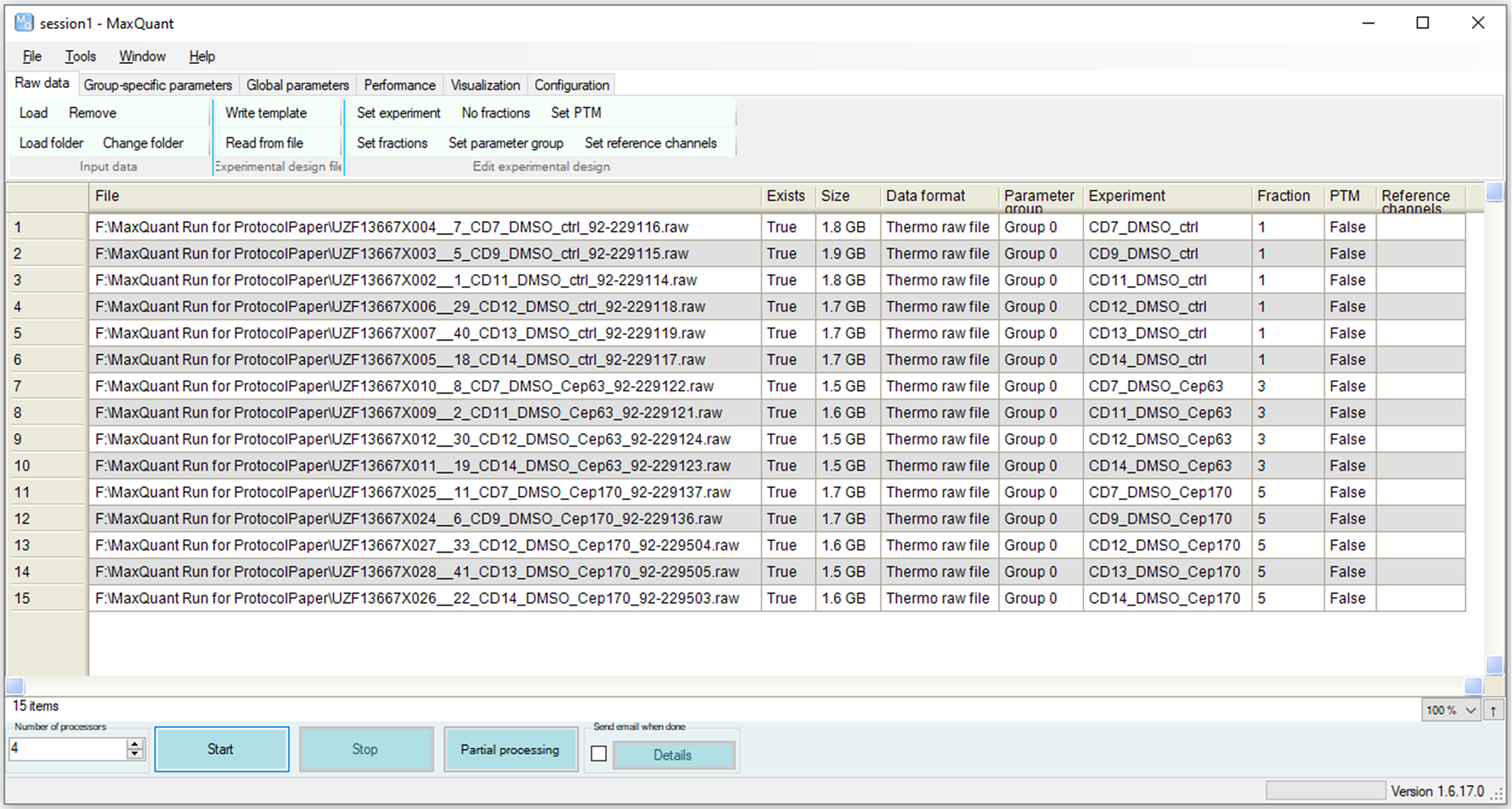
      Figure 10. Example experimental design for a MaxQuant run

      
      

      BOX1: Matching between runs In cases where some of the peptide sequences could not be identified from the MS/MS spectrum due to insufficient information, missing values can be compensated by matching the run with another, to still get identified features (Tyanova et al., 2016). Matching should be done only between similar samples and the MaxQuant algorithm matches only between the same or adjacent fractions. TIP: Because it is not expected to have a very similar set of proteins pulled down by different antibodies in co-IPs, unlike the total proteome, we aimed to match only replicate samples. This is done by a trick to assign the biological replicate IPs to the same fraction and skipping a number for the next set of IPs, to minimize false positives, while facilitating recovery of unidentified peaks using replicate IPs (Figure 10).

      
      

      1. Manual setup:

         i. Assign fractions.

         1) Select the replicate IPs by Ctrl+left-click.

         2) Raw data > Edit experimental design > Set fractions (Figure 11).

         
         

         
         Figure 11. Assigning fractions to a sample (write the same number to both fields)

         
         

         ii. Assign experiment names:

         Select the sample > Raw data > Edit experimental design > Set experiment > and give a unique experiment name to each sample.

      2. Alternatively, assign parameters in bulk using Excel:

         i. Raw data > Experimental design file > Write template.

         ii. Find the file: experimentalDesignTemplate.txt in the >combined folder and open with Excel.

         iii. Assign a unique experiment name to each sample (e.g., Text-to-column function can be used to generate them from sample names). Assign the same fraction number to replicate samples and skip at least one number for the next set of replicates (e.g., all controls: 1, all CEP63 IPs: 3) (see “Fraction” in Figure 10).

         iv. Save the file (as .txt) and upload via Raw data > Experimental design file > Read from file > locate the experimentalDesignTemplate.txt (MaxQuant Analysis Files).

   7. Provide the sequence database to be used for peptide identification.

      1. Global parameters > Parameter section > Sequences.

      2. Fasta files: Add > Locate the .fasta file to be used:

         The reviewed human protein reference can be retrieved from UniProt database as follows:

         i. Go to https://www.uniprot.org > Proteins.

         ii. Select Human and Status: “Reviewed” (Swiss-Prot).

         iii. Download (all) > Format: FASTA (canonical & isoform).

         Taxon identifier: 9606 (Homo sapiens), canonical sequences and isoforms (reviewed), 15th June 2021 was used for the current protocol (MaxQuant Analysis Files: 2021_02_Human_canonical_and_isoforms.fasta).

      3. Select the uploaded file on the software (Fasta file path) and select > Identifier rule > UniProt identifier: >.*\|(.*)\|

   8. Click Start at the bottom of the software.

      Depending on the experiment size and the computing power, the run can take from a few days to more than a week.

   9. The results can be found in the “combined” folder that is placed in the same folder with .RAW files. combined > txt > proteinGroups.txt will be used for the subsequent Perseus analysis.

      
      

   Part II: Perseus analysis

   2. Pre-processing, annotation, and quality control (TIMING: 0.5–2 days)

      Notes:

      1. Protein interactors of the baits were determined by processing the MaxQuant result table ProteinGroups.txt in Perseus software (Tyanova et al., 2016). Tutorial pages and videos can be found at http://coxdocs.org/doku.php?id=perseus:start. Please note that Perseus can currently run only on Windows operating systems.

      2. Perseus software generates a new matrix for each step; therefore, always apply the next operation to the latest matrix generated.

      3. It is possible to re-color or re-name a matrix by right-clicking on it, which would be helpful especially for long workflows.

      4. Matrices can be deleted using the red cross mark at the top of the section where the workflow tree is.

      5. The workspace can be saved at any point and can be resumed later.

      
      

      CRITICAL: The .sps files generated in one version of Perseus cannot be processed using another version. Therefore, we strongly recommend to always record the version number and keep a copy of the software together with the analysis files.

      TIP: It is advised to save the Perseus file frequently to avoid data loss due to occasional software crash.

      1. Download the Perseus software.

         1. Latest version can be found under: https://maxquant.net/download_asset/perseus/latest. Perseus version 1.6.14.0 (Supplementary information) was used in the original research described in O’Neill et al. (2022) and for the current protocol.

         2. Initiate the software by double-clicking on Perseus.exe (no installation is required) [Perseus Analysis Files: 1_ExampleAnalysis_Part1.sps]

      2. Import the MaxQuant results table into Perseus:

         1. For this protocol, the following example dataset was used:

            i. Negative controls:

            1) UZF13667X004__7_CD7_DMSO_ctrl_92-229116.raw

            2) UZF13667X003__5_CD9_DMSO_ctrl_92-229115.raw

            3) UZF13667X002__1_CD11_DMSO_ctrl_92-229114.raw

            4) UZF13667X006__29_CD12_DMSO_ctrl_92-229118.raw

            5) UZF13667X007__40_CD13_DMSO_ctrl_92-229119.raw

            6) UZF13667X005__18_CD14_DMSO_ctrl_92-229117.raw

            ii. CEP63 IPs

            1) UZF13667X010__8_CD7_DMSO_Cep63_92-229122.raw

            2) UZF13667X009__2_CD11_DMSO_Cep63_92-229121.raw

            3) UZF13667X012__30_CD12_DMSO_Cep63_92-229124.raw

            4) UZF13667X011__19_CD14_DMSO_Cep63_92-229123.raw

            iii. CEP170 IPs:

            1) UZF13667X025__11_CD7_DMSO_Cep170_92-229137.raw

            2) UZF13667X024__6_CD9_DMSO_Cep170_92-229136.raw

            3) UZF13667X027__33_CD12_DMSO_Cep170_92-229504.raw

            4) UZF13667X028__41_CD13_DMSO_Cep170_92-229505.raw

            5) UZF13667X026__22_CD14_DMSO_Cep170_92-229503.raw

         2. Click on Matrix > Load > Generic matrix upload (green arrow pointing upper left).

         3. File: Select > locate the MaxQuant results folder: combined > txt > proteinGroups.txt [Perseus Analysis Files: 2_proteinGroups.txt]

         4. Include columns by selecting the items on the left menu and transferring to the respective category on the right using arrows. TIP: Holding down Ctrl button and/or left clicking and pulling down allows multiple selection. The order of items within the category can be changed using up and down arrows on the right side. We included columns we marked as “optional” in the initial upload, and then removed, in case some parameters must be retrospectively checked during the analysis, to avoid starting all over again. [ExampleAnalysis_Part1: Full Matrix]

            i. Main (experimental quantitative results)

            1) LFQ intensity (for each sample)

            2) iBAQ (for each sample)

            3) Intensity (for each sample)

            ii. Numerical

            1) Peptides

            2) Razor + unique peptides

            3) Unique peptides

            4) Optional: Sequence coverage [%]

            5) Optional: Unique + razor sequence coverage [%]

            6) Optional: Unique sequence coverage [%]

            7) Mol. weight [kDa]

            8) Q-value

            9) Score

            10) Optional: Intensity

            11) Optional: iBAQ peptides

            12) MS/MS count

            13) Number of proteins

            14) Optional: Unique peptides (for each sample)

            15) Optional: Peptides (for each sample)

            16) Optional: Razor + unique peptides (for each sample)

            17) Optional: MS/MS count (for each sample)

            iii. Categorical

            1) Only identified by site

            2) Reverse

            3) Potential contaminant

            4) Optional: Identification type (for each sample)

            iv. Text

            1) Protein IDs

            2) Majority protein IDs

            3) Protein names

            4) Gene names

            5) Fasta headers

            v. Multi-numerical

            1) Peptide counts (all)

            2) Peptide counts (razor+unique)

            3) Peptide counts (unique)

         5. Remove optional columns to avoid large file size during subsequent analyses [ExampleAnalysis_Part1: Smaller Matrix].

            i. Left-click on the matrix and select on the menu: Matrix > Processing > Rearrange > Reorder/remove columns.

            ii. Select the items on the right menu and transfer the respective category back to the left.

      3. Add different categories to the samples to be able to group them for statistical analysis.

         1. It is possible to add annotation rows manually:

            i. Matrix > Processing > Annot. rows > Categorical annotation rows.

            ii. Action: Create.

            iii. Row name: Assign a name to the category.

            iv. Add categories to each sample.

         2. Alternatively, add all annotations at once for a large number of samples and multiple categories, editing the template file in Excel:

            i. First, create a mock annotation row following the steps above (this is required for exporting the template file) [ExampleAnalysis_Part1: Placeholder Category].

            ii. Then, export to a matrix:

            1) Matrix > Processing > Annot. rows > Extract to matrix [ExampleAnalysis_Part1: Placeholder Annotation].

            2) Select the new matrix and Matrix > Generic matrix export (upper rightmost, floppy disc icon) > click on the Select button to choose the folder, assign a file name, and click OK.

            iii. Open the file in Excel and create a new column (letter “C” should be assigned as the column type, meaning “Categorical”) for each category to be added (TIP: Original column names can be chopped using Data Tools > Text to Columns and combined in different ways to generate categories) (Table 2). Here, we generated the following categories:

            1) Experiment: DMSO_ctrl_CD7, DMSO_CEP63_CD11, …

            2) Measurement: LFQ, iBAQ, Intensity

            3) IP: ctrl, CEP63, CEP170

            4) Replicate: CD7, CD9, CD11, CD12, CD13, CD14

            5) IP_Rep: ctrl_CD7, ctrl_CD9, CEP63_CD7, …

            
            

            Table 2. An example annotation file

            Experiment	Measurement	IP	IP_Rep	Name
            #!{Type}C	C	C	C	T
            DMSO_ctrl_CD7	LFQ	ctrl	ctrl_CD7	LFQ intensity CD7_DMSO_ctrl
            DMSO_CEP63_CD7	LFQ	CEP63	CEP63_CD7	LFQ intensity CD7_DMSO_Cep63
            DMSO_CEP170_CD12	LFQ	CEP170	CEP170_CD12	LFQ intensity CD12_DMSO_Cep170
            DMSO_ctrl_CD7	iBAQ	ctrl	ctrl_CD7	iBAQ CD7_DMSO_ctrl
            DMSO_CEP63_CD7	iBAQ	CEP63	CEP63_CD7	iBAQ CD7_DMSO_Cep63
            DMSO_CEP170_CD12	iBAQ	CEP170	CEP170_CD12	iBAQ CD12_DMSO_Cep170
            DMSO_ctrl_CD7	Intensity	ctrl	ctrl_CD7	Intensity CD7_DMSO_ctrl
            DMSO_CEP63_CD7	Intensity	CEP63	CEP63_CD7	Intensity CD7_DMSO_Cep63
            DMSO_CEP170_CD12	Intensity	CEP170	CEP170_CD12	Intensity CD12_DMSO_Cep170

            iv. Rename the cell “Column name” as “Name” (otherwise Perseus generates an error) and save as a .txt file [Perseus Analysis Files: 3_Categories.txt].

            v. Go back to Perseus, select the last matrix before exporting annotations (Smaller Matrix), and go to Matrix > Processing > Annot. rows > Categorical annotation rows > Action: Read from file > Input file: locate the saved annotation file using the Select button [ExampleAnalysis_Part1: Added: Categories].

      4. Filter the annotated matrix based on MaxQuant quality parameters.

         1. Matrix > Processing > Filter rows > Filter rows based on categorical column (Figure 12).

            
            

            
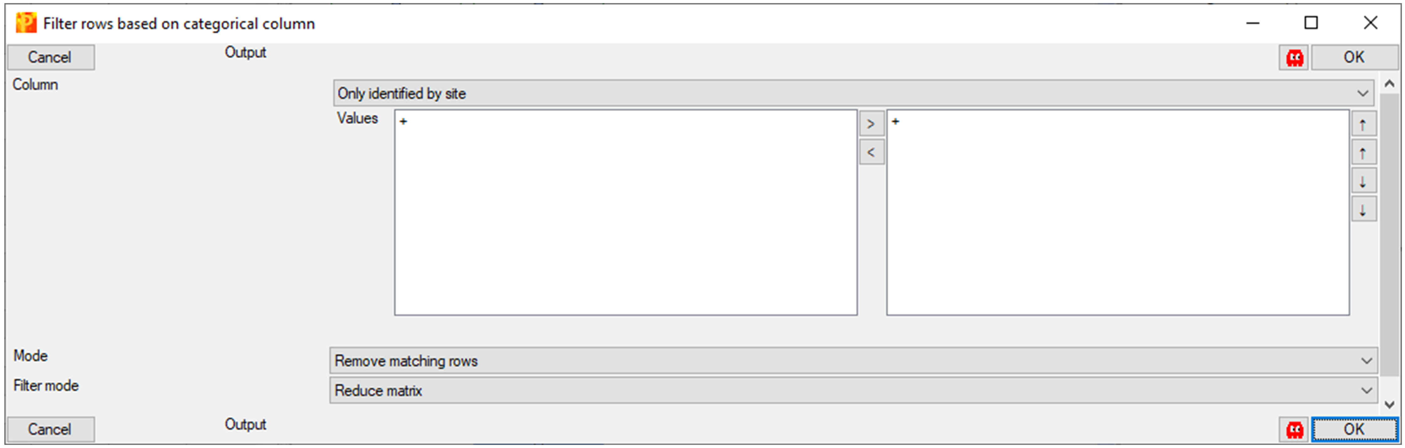
            Figure 12. Filtering rows based on a categorical column

            
            

            i. Column: Only identified by site (these proteins did not go through proper FDR, because they were identified by only peptides with modified amino acids).

            1) Values: + (on the right side).

            2) Mode: remove matching rows.

            3) Filter mode: Reduce matrix.

            4) Click OK.

            ii. Column: Reverse (sequences found in reverses decoy database, which is used to calculate the FDR, i.e., statistical cutoff for acceptable spectral matches).

            1) Values: + (on the right side).

            2) Mode: remove matching rows.

            3) Filter mode: Reduce matrix.

            4) Click OK.

            iii. Column: Potential contaminant (proteins that are commonly occurring contaminants in the mass spectrometry data).

            1) Values: + (on the right side).

            2) Mode: remove matching rows.

            3) Filter mode: Reduce matrix.

            4) Click OK.

            Optional: Check whether anything filtered out looks important using “Split matrix” instead.

         2. Filter out immunoglobulins (these can come from the antibodies used for co-immunoprecipitation):

            Matrix > Processing > Filter rows > Filter rows based on text column > Column: Fasta headers

            i. Search string: “immunoglobulin.”

            ii. Deselect Match whole word.

            iii. Mode: Remove matching rows.

            iv. Filter mode: Reduce matrix.

            v. Click OK.

            Optional: Check whether anything filtered out looks important using “Split matrix” instead.

      5. Optional: Add pathway annotations (e.g., KEGG pathway, GO terms); this can also be done later.

         1. Download the annotations:

            i. Tools > Annotation download >http://annotations.perseus-framework.org> PerseusAnnotation

            1) > FrequentlyUsed > mainAnnot.homo_sapiens.txt.gz.

            2) Can also be found under: > OrganismSpecific > h > scroll down to find Homo sapiens.

            ii. Download and place the file (no need to extract) into the folder location: Perseus 1.6.14.0 > bin > conf > annotations.

         2. Add the annotations:

            Matrix > Processing > Annot. columns > Add annotation.

            i. Source: select mainAnnot.homo_sapiens.txt.gz (it should now be automatically listed).

            ii. UniProt column: Protein IDs.

            iii. Add the annotations of your interest, e.g.:

            1) GOBP name

            2) GOMF name

            3) GOCC name

            4) KEGG name

            5) Corum

      6. Export the matrix as a backup before the next step of the analysis: Matrix > Export > Generic Matrix Export > AfterBasicFilters.txt.

         1. Correct the missing protein names or gene symbols that might be converted to date because of opening the file in Excel (e.g., SEPTINs, MARCs) (Figure 13).

            
            

            
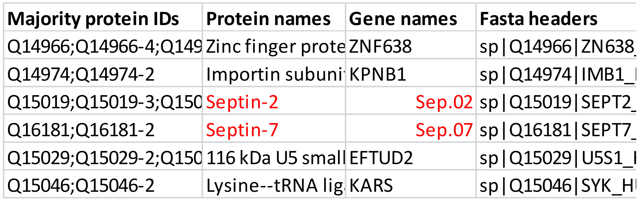
            Figure 13. Pay attention to the protein names; these might be converted to dates when the files are processed in Excel

            
            

         2. Further potentially problematic protein names include: CALM3 (Calmodulin-3, P0DP25), PBX3, CV015, TMM70, CC201, CRCC2, TPM1, TPM3, MIC60, MACF1, ZN683, HNF4A, ASCC1, and SREK1 (e.g., missing protein names or gene names).

         3. After correcting, save as .txt file [Perseus Analysis Files: 4_AfterBasicFilters.txt].

      7. Cluster analysis (using Perseus and R software):

         1. Perseus

            i. Upload the corrected AfterBasicFilters.txt file: Matrix > Load > Generic matrix upload.

            ii. Pre-processing:

            1) Transform the data [ExampleAnalysis_Part1: log2 (x+1)]: Log2-transformation: Matrix > Processing > Basic > Transform

            a) Transformation: log2(x+1).

            b) Columns: select all the main columns.

            2) Subset the LFQ Intensities: Matrix > Processing > Rearrange > Reorder/remove columns.

            3) Transfer the iBAQ and Intensity columns back to left side and keep as the main columns only LFQ Intensities [ExampleAnalysis_Part1: LFQ]

            iii. Filter out the proteins detected in less than two samples in total:

            1) Matrix > Processing > Filter rows > Filter rows based on valid values.

            2) Min. valids > Number: 2.

            3) Mode: In total.

            4) Values should be > Greater than: 0.

            5) Filter mode: Reduce matrix.

            iv. PCA Analysis (Figure 14): Matrix > Analysis > Principal component analysis (the symbol with red and blue dots).

            
            

            
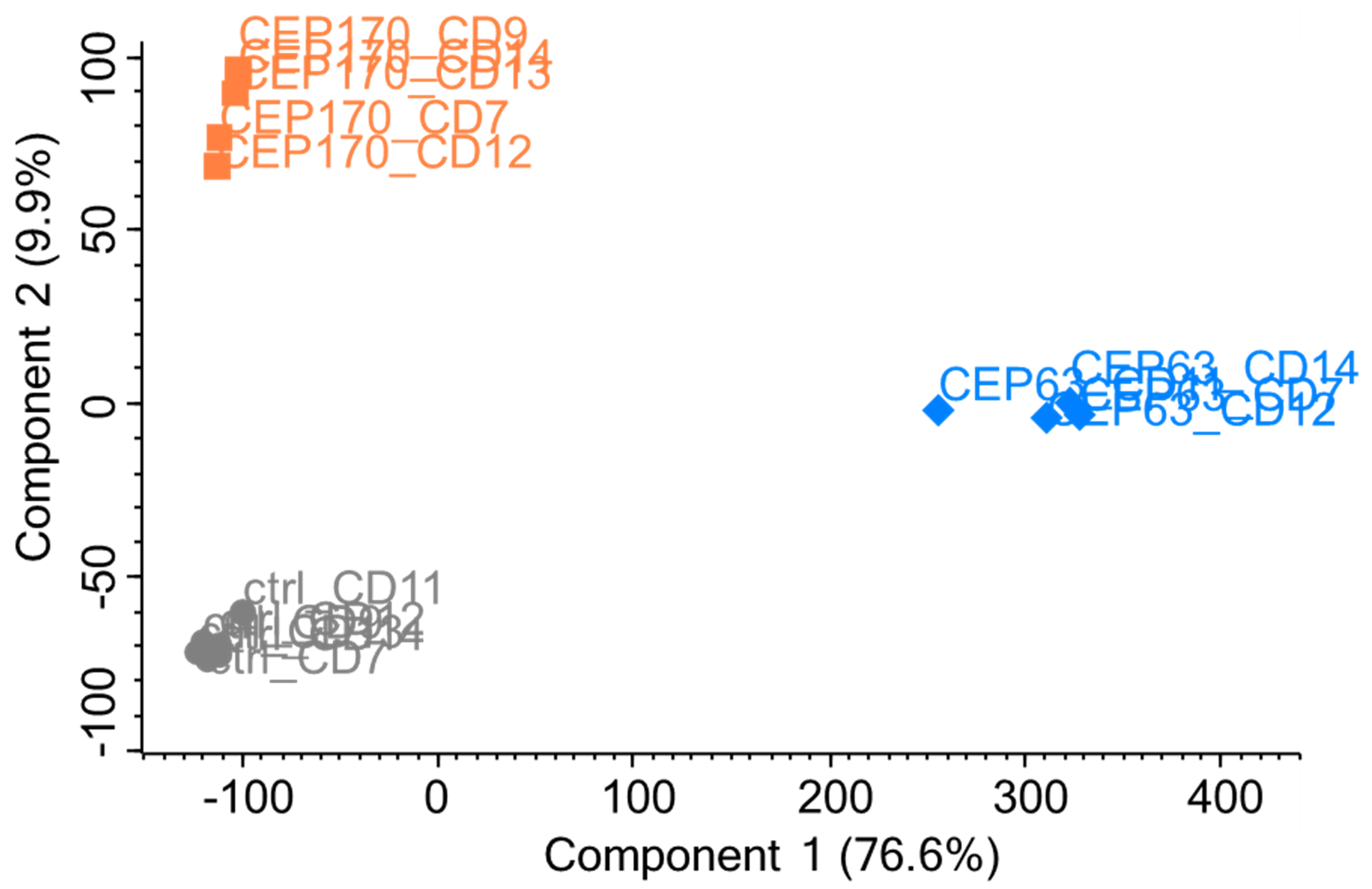
            Figure 14. PCA analysis (LFQ Intensities)

            
            

            1) Labels can be made visible from: Points tab > Right-click on the data > Select all > Show labels (gray label sign on top). Label text can be changed using the menu item on top of the plot.

            2) Replicates can be colored using the menu in the Points and Categories tabs of the PCA.

            3) Symbol type, size, and color can be modified.

            v. Hierarchical clustering (Figure 15): Matrix > Analysis > Hierarchical clustering.

            1) Default settings can be used.

            2) Appearance of the heatmap can be adjusted using the menu items on the Heat Map tab (size, labels to show, colors etc.) (Figure 16).

            
            

            
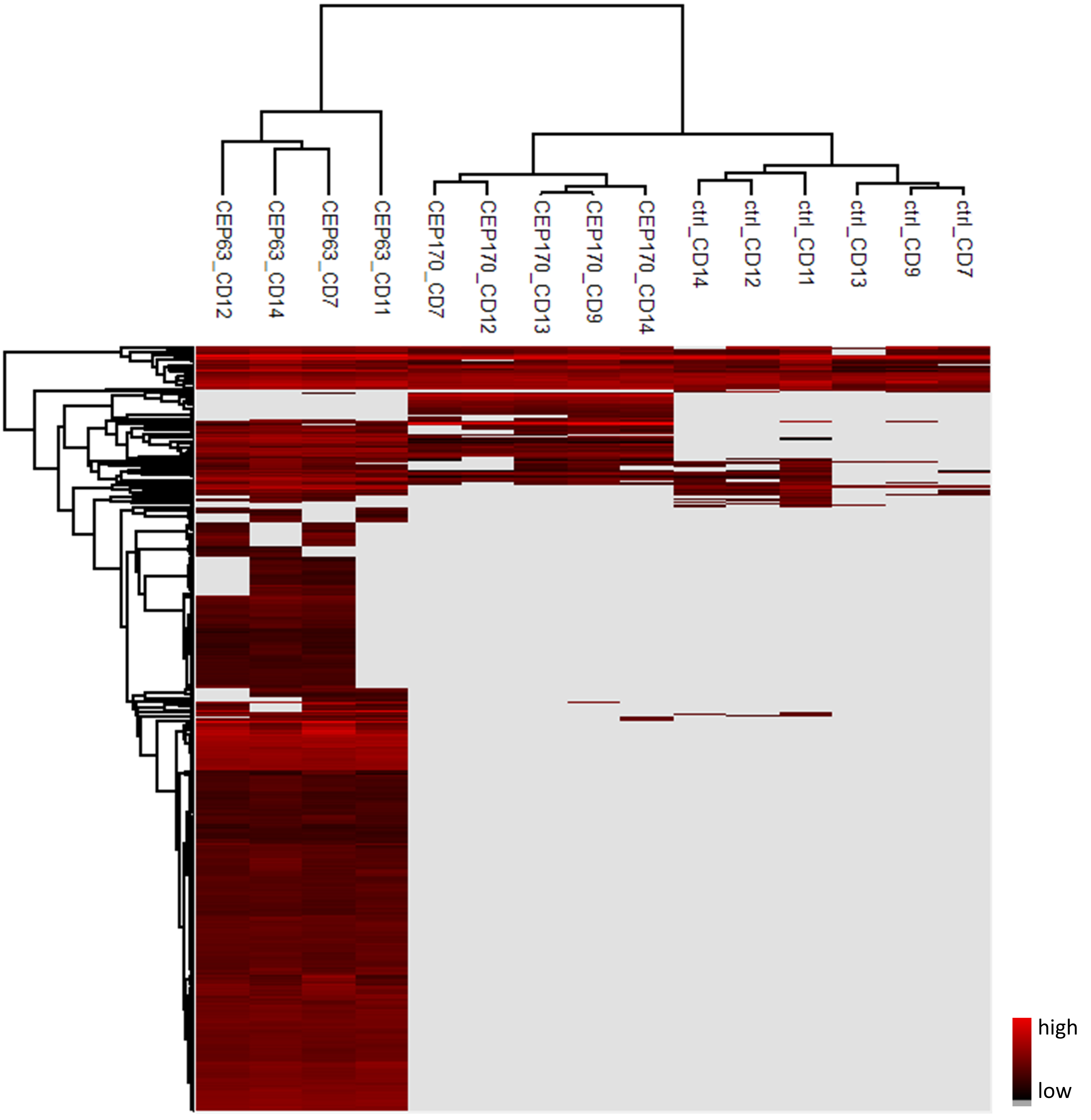
            Figure 15. Hierarchical clustering of the samples in the current analysis (LFQ Intensities)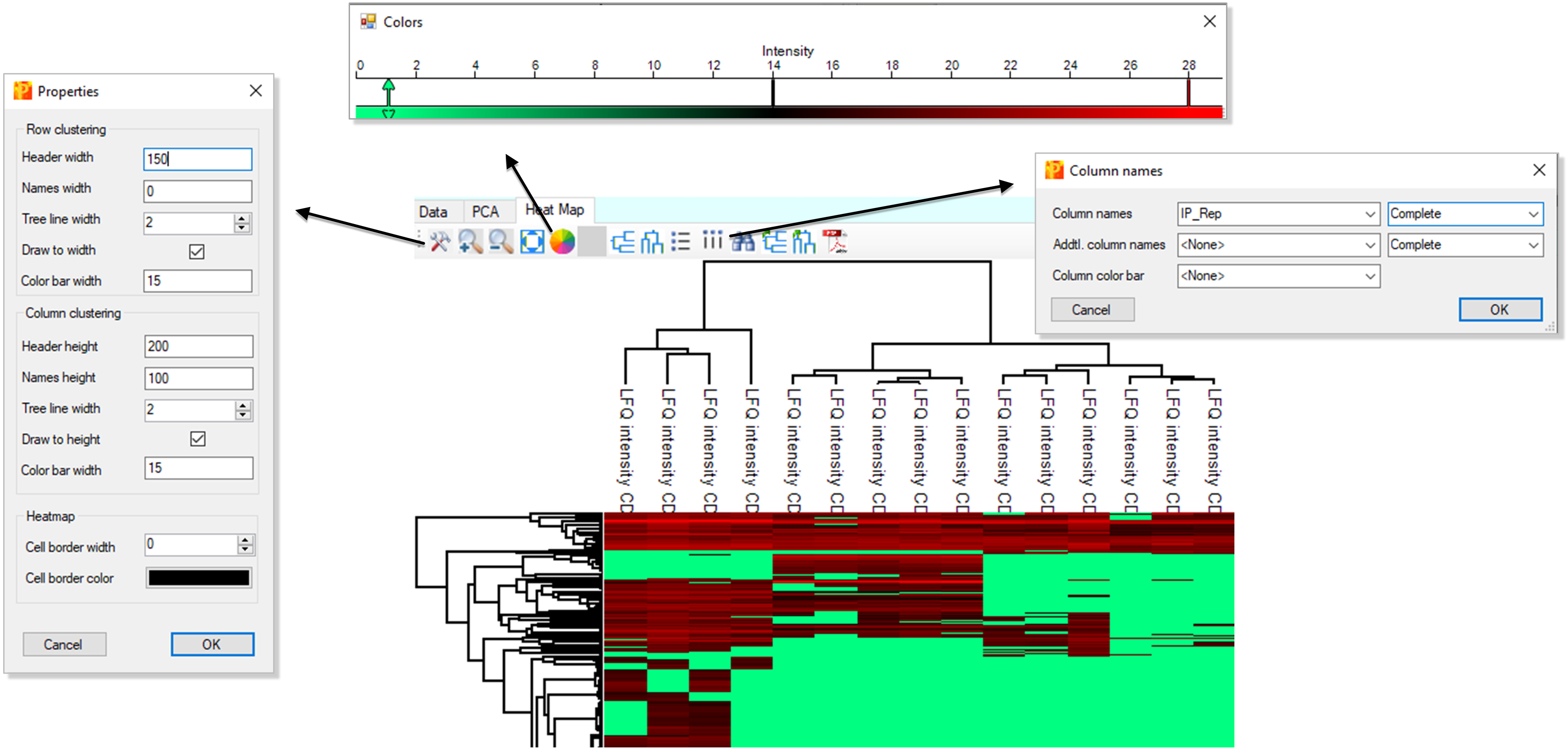

            
            

            
            Figure 16. Appearance of the heatmap can be adjusted using menu items in the menu

            
            

         2. Dimensionality reduction analysis using R statistical software:

            i. Export the matrix filtered for PCA analysis: Matrix > Export > Generic Matrix Export > Select: LFQ.txt [Perseus Analysis Files: 5_LFQ.txt].

            ii. Refer to the sample R script 6_Cluster_Analysis.R (Perseus Analysis Files).

            iii. Run tSNE and UMAP analysis using R (Figure 17).

            
            

            
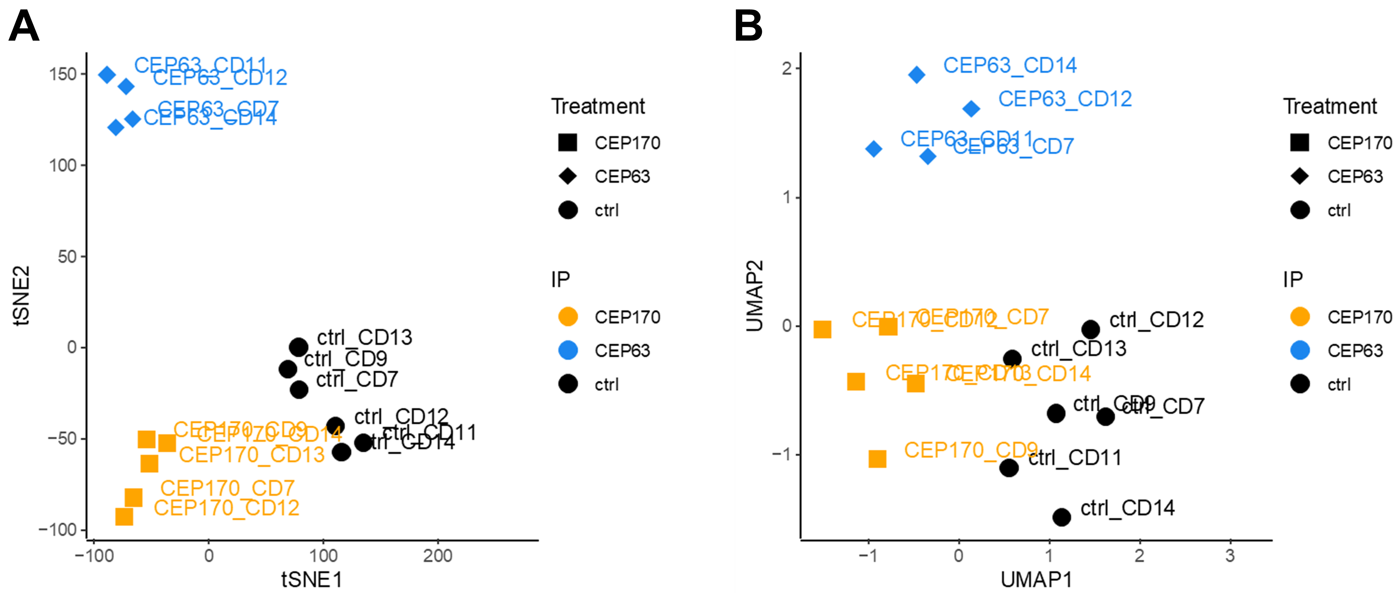
            Figure 17. tSNE and UMAP visualization (LFQ Intensities)

            
            

      3. Statistical analysis (TIMING: 2–7 days, depending on the number of samples)

         Note: Here, we provide one approach among many possibilities for statistical analysis; alternative tests or methods can also be used for evaluation of the enriched proteins.

         1. Create a separate .sps file per bait, starting with the AfterBasicFilters matrix. In this example, we generated the following two files:

            1. Perseus Analysis Files: 8_ExampleAnalysis_Part2_CEP63.sps.

            2. Perseus Analysis Files: 9_ExampleAnalysis_Part2_CEP170.sps.

         2. Run t-test in Perseus (volcano plot):

            1. Import filtered and corrected data [Perseus Analysis Files: 4_AfterBasicFilters.txt]: Matrix > Load > Generic matrix upload >

            2. Transform the data [ExampleAnalysis_Part2_CEP63: log2 (x+1)]

               i. Log2-transformation: Matrix > Processing > Basic > Transform

               ii. Transformation: log2(x+1)

            3. Subset the LFQ intensities as a new matrix to run the statistical test [ExampleAnalysis_Part2_CEP63: CEP63 LFQ]. Matrix > Processing > Rearrange > Reorder/remove columns > keep only the LFQ Intensities of the bait of interest and the negative controls and transfer the rest of the main columns to the left. For example, the new matrix may contain the following main columns:

               i. LFQ Intensity CD7_DMSO_ctrl

               ii. LFQ Intensity CD9_DMSO_ctrl

               iii. LFQ Intensity CD11_DMSO_ctrl

               iv. LFQ Intensity CD12_DMSO_ctrl

               v. LFQ Intensity CD13_DMSO_ctrl

               vi. LFQ Intensity CD14_DMSO_ctrl

               vii. LFQ Intensity CD7_DMSO_Cep63

               viii. LFQ Intensity CD11_DMSO_Cep63

               ix. LFQ Intensity CD12_DMSO_Cep63

               x. LFQ Intensity CD14_DMSO_Cep63

            4. Optional: Remove any outlier samples, if necessary.

               i. Following plots can be used for determining the outliers:

               1) PCA plot.

               2) Profile plot (i.e., box plot).

               3) Multi-scatter plot.

               4) tSNE/UMAP (R software).

               ii. Matrix > Processing > Rearrange > Reorder/remove columns > transfer respective outlier column(s) to the left, if any.

            5. Filter out the proteins detected in less than two replicates [ExampleAnalysis_Part2_CEP63: Filtered: 2+ valid].

               Matrix > Processing > Filter rows > Filter rows based on valid values.

               i. Min. valids > Number: 2.

               ii. Mode: In at least one group.

               iii. Grouping: IP (one of your annotations).

               iv. Values should be > Greater than: 0.

               v. Filter mode: Reduce matrix.

            6. Apply t-test (unpaired one-tailed Student’s t-test): Matrix > Analysis > Volcano plot.

               i. Grouping: IP.

               1) First group (right): CEP63.

               2) Second group (left): ctrl.

               ii. Test: t-test.

               iii. Side: Left.

               iv. Number of randomizations: 1,000.

               v. FDR: 0.1, S0: 10 (initial settings).

         3. Rank the proteins into statistical significance categories using π-value (Xiao et al., 2014):

            1. Transfer the data to an Excel file.

               In the table part of volcano plot: Points > Right-click on the data > Select all > Right-click on the data.

               i. > Copy selected rows > paste to an Excel file.

               ii. Alternatively: > Plain matrix export… > .txt which can then be imported into Excel as a tab delimited file.

            2. In Excel, calculate the π-values [Perseus Analysis Files: 10_π-values.xlsx].

               Create a new column and calculate -log(p-value) × Difference.

               i. Should be 2^nd and 3^rd columns. -log(p-value) column might be converted to #NAME?

               ii. “Difference” corresponds to fold-change.

            3. Sort the proteins based on the π-values:

               i. Using the natural separation of the π-values on the plot (Figure 18), set thresholds.

               In this case, we used around 100, 30, 12, and 8:

               1) Score 4: 100 > π-value

               2) Score 3: 100 > π-value > 30

               3) Score 2: 30 > π-value > 12

               4) Score 1: 12 > π-value > 8

               ii. Regardless of its π-value, DO NOT accept anything with:

               1) Difference (fold-change) < 5

               2) -log(p-val) < 0.9

               iii. The FDR and S0 values in the volcano plot corresponding to these cut-offs in this case were:

               1) CEP63: FDR: 0.03, S0: 10

               2) CEP170: FDR: 0.06, S0: 10

               iv. Go back to Perseus, and color the proteins on the volcano plot according to the scores:

               1) CRITICAL: These colors will subsequently be used in the R script to assign scores. Therefore, make sure to use the exact same colors across analyses.

               2) TIP: It can be helpful to search the highest and lowest few proteins of a given score in the volcano plot, color them first, and then color the ones that fall in between.

               
               

               
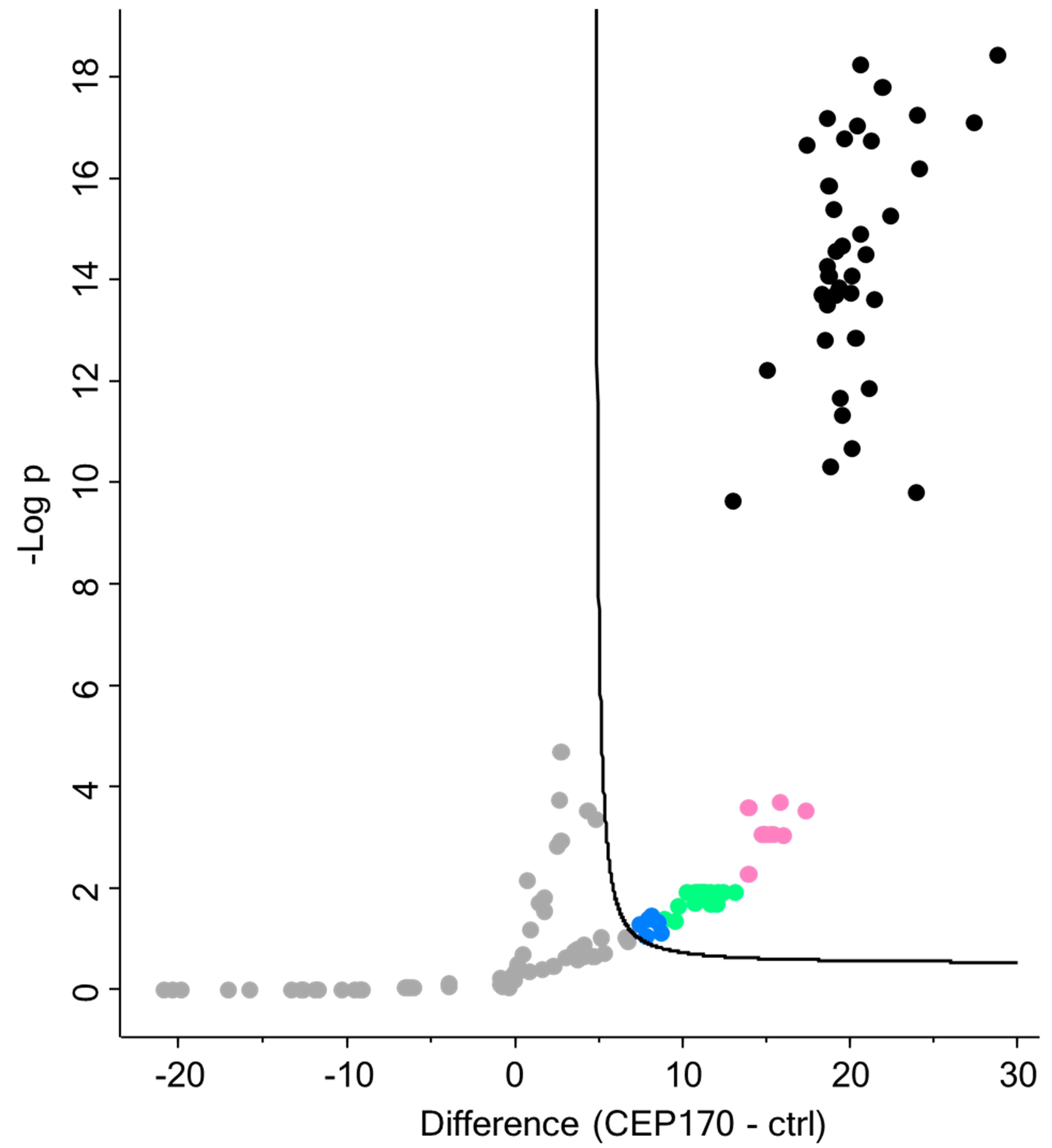
               Figure 18. Volcano plot of the proteins ranked and colored based on π-value. From highest to lowest rank: ● Score 4; ●Score 3; ● Score 2; ● Score 1

               
               

         4. Transfer the significant ranked values to Excel:

            1. First, select all the non-colored (gray) points; then, invert the selection to keep the colored (significant) ones, as follows:

               i. In the table part of volcano plot: Points >.

               ii. Click on a gray (non-colored) dot in the “Symbol color” column and copy the value shown below the table [i.e., default value: Color2 (A = 255, R = 169, G = 169, B = 169)].

               iii. Right-click on the data:

               1) > Find…: Color2 [A = 255, R = 169, G = 169, B = 169].

               2) > Look in: Symbol color.

               3) > Find all > Right-click on the rows > Select all and close this window.

               iv. Points > Right-click on the data > Invert selection. Now, all the significant, colored (non-gray) points should be selected.

               v. Right-click on the data > Copy selected rows.

               vi. Paste the copied data to the Excel file, corresponding tab [Perseus Analysis Files: 11_Selection_from_Volcano.xlsx].

               1) Create a separate tab for each bait analyzed.

               2) Rename the “-Log(p-Value)” column (which might be changed to “#NAME?” by Excel) as “minus_log10_p”.

               3) Correct the Septins and other problematic gene names (mentioned in section B6 and Figure 13) if converted to date.

               
               

         Part III. Further analysis

         4. Combine and summarize the data (TIMING: 0.5 day)

            1. Combine and clean-up the data saved in Selection_from_Volcano.xlsx using R [Perseus Analysis Files: 12_Tidy_Data.R]. This script generates two Excel files:

            2. Significant_Final.xlsx. Each tab of this file lists the proteins enriched by one bait, including Gene names, Protein IDs, Protein names, -log(p-value), log(fold-change) (i.e., Difference), and significance score (4: highest, 1: lowest).

            3. Significant_Final_Frequencies.xlsx. This table summarizes by how many baits each protein was pulled down and with which score.

               
               

         5. Further analysis suggestions (TIMING: variable)

            1. Networks can be generated using bait-protein pairwise interactions using the Cytoscape software: https://cytoscape.org/.

            2. Protein-protein interactions among the interactors of the baits can be analyzed for Gene Ontology (GO) terms using STRING database: https://string-db.org/.

               Use the Multiple proteins search option and use the Gene.names2 column of the Significant_Final.xlsx file for the search, as it lists single protein names instead of protein groups.

Recipes

Note: For the solutions that require pH adjustment, use initially ~60%–80% of the volume of the water to solve the reagents, and complete the volume only after adjusting the pH.

1. 2 M NaCl

   Reagent	MW	Quantity
   NaCl	58.44 g/mol	23.376 g
   Distilled water
   Final		200 mL

   *Can be kept at room temperature.

   
   

2. 0.5 M EDTA, pH 7.5

   Reagent	MW	Quantity
   EDTA	292.24 g/mol	14.612 g
   Distilled water
   Final		100 mL

   *Dissolves after adding NaOH pellets and warming, pH 7.5. Can be kept at room temperature.

   
   

3. 0.5 M EGTA, pH 7.6

   Reagent	MW	Quantity
   EGTA	380.35 g/mol	19.018 g
   Distilled water
   Final		100 mL

   *Dissolves after adding NaOH crystals and warming, pH 7.6. Can be kept at room temperature.

   
   

4. 1 M Tris-HCl, pH 7.5

   Reagent	MW	Quantity
   Tris base	121.14 g/mol	24.228 g
   Distilled water
   Final		200 mL

   *Adjust the pH to 7.5 with concentrated HCl. Can be kept at room temperature.

   
   

5. 0.5 M Tris-HCl, pH 6.8

   Reagent	MW	Quantity
   Tris base	121.14 g/mol	12.11 g
   Distilled water
   Final		200 mL

   *Adjust the pH to 6.8 with concentrated HCl. Can be kept at room temperature.

   
   

6. 10% Triton X-100 (v/v)

   Reagent	Stock	Final concentration	Quantity
   Triton X-100	100%	10%	20 mL
   Distilled water			180 mL
   Final			200 mL

   *Can be kept at room temperature.

   
   

7. 10% SDS (w/v)

   Reagent	MW	Quantity
   SDS (powder)	288.372 g/mol	10 g
   Distilled water, up to		100 mL
   Final		100 mL

   *Can be kept at room temperature.

   
   

8. ROCK inhibitor, 10 mM

   Reagent	MW	Quantity
   Y-27632 (dihydrochloride), powder	320.3 g/mol	5 mg
   Water, sterile		1.56 mL
   Final		1.56 mL

   *Aliquot and keep at -20 °C. Once thawed, the vial can be kept at 4 °C.

   
   

9. Dorsomorphin, 5 mM

   Reagent	MW	Quantity
   Dorsomorphin, powder	399.5 g/mol	5 mg
   DMSO, sterile		2.5 mL
   Final		2.5 mL

   *Observe the solution closely when dissolving dorsomorphin and look for floating tiny particles. If it is not dissolved completely, try warming up to 37 or 50 °C for 15–20 min. Aliquot and keep at -20 °C. Once thawed, the vial can be kept at 4 °C.

   
   

10. SB431542, 10 mM

    Reagent	MW	Quantity
    SB431542 hydrate, powder	384.39 g/mol	5 mg
    DMSO, sterile		1.3 mL
    Final		1.3 mL

    *Aliquot and keep at -20 °C. Once thawed, the vial can be kept at 4 °C.

    
    

11. Nocodazole, 3.3 mM

    Reagent	MW	Quantity
    Nocodazole, powder	301.32 g/mol	2 mg
    DMSO, sterile		2.0114 mL
    Final		2.0114 mL

    *Aliquot and keep at -20 °C. Thawed vial can be re-frozen and used a few times.

    
    

12. Poly-L-Ornithine, 10 mg/mL

    Reagent	MW	Quantity
    Poly-L-Ornithine hydrobromide, powder	30–70 kDa	500 mg
    Water, sterile		50 mL
    Final		50 mL

    *Aliquot and keep at -20 °C. Once thawed, the vial can be kept at 4 °C.

    
    

13. Neural maintenance medium (N3)

    Reagent	Stock	Dilution	Final concentration	Volume
    DMEM/F-12, GlutaMAXTM supplement		~1:2	~0.5×	241 mL
    Neurobasal medium (1×) [-] L-Glutamine		~1:2	~0.5×	241 mL
    B27 with vitamin A	50×	1:100	0.5×	5 mL
    Penicillin-Streptomycin	100×	1:100	1×	5 mL
    N2 supplement	100×	1:200	0.5×	2.5 mL
    Non-essential amino acids	100×	1:200	0.5×	2.5 mL
    GlutaMAXTM supplement	100×	1:200	0.5×	2.5 mL
    2-mercaptoethanol	50 mM	1:1,000	50 μM	500 μL
    Insulin	10 mg/mL	1:4,000	2.5 μg/mL	125 μL
    Final				500 mL

    *Filter media using a 0.22 μm vacuum filter. N3 medium can be stored for up to three weeks at 4 °C.

    
    

14. Neural induction medium (N3+SMADi)

    Reagent	Stock	Dilution	Final concentration	Volume
    Neural maintenance medium (N3)	-	-	-	50 mL
    SB431542	10 mM	1:1,000	10 μM	50 μL
    Dorsomorphin	5 mM	1:5,000	1 μM	10 μL
    Final				50 mL

    * After adding SMAD inhibitors (i.e., as N3+SMADi), keep the medium at 4 °C and use within five days.

    
    

15. Protein standard (BSA) (64 mg/mL)

    Reagent	Stock
    BSA	320 mg
    IP/wash buffer	5 mL
    Final	5 mL

    *Aliquot and keep at -20 °C. Thawed vial can be re-frozen and used a few times.

    
    

16. 1× Laemmli buffer

    Reagent	Stock	Final concentration	Volume
    Tris-HCl, pH 6.8	0.5 M	32.9 mM	658 μL
    SDS	10%	1%	1 mL
    Distilled water			8.092 mL
    Final			9.75 mL

    *Stable at room temperature for six months. Mix with 2-mercaptoethanol at 39:1 ratio as a small aliquot just before using (e.g., 975 μL of 1× Laemmli + 25 μL of 2-mercaptoethanol).

    
    

17. IP/wash buffer A

    Reagent	Stock	Final concentration	Volume
    Distilled water			38.05 mL
    Tris-HCl, pH 7.5	1 M	50 mM	2.5 mL
    NaCl	2 M	150 mM	3.75 mL
    EDTA	0.5 M	1 mM	100 μL
    EGTA, pH 7.6	0.5 M	1 mM	100 μL
    Triton X-100	10%	1%	5 mL
    SDS	10%	0.1%	500 μL
    Protease inhibitor			1 tablet
    Final			50 mL

    *Make fresh on the day of use.

    
    

18. Wash buffer B

    Reagent	Stock	Final concentration	Volume
    Distilled water			43.55 mL
    Tris-HCl, pH 7.5	1 M	50 mM	2.5 mL
    NaCl	2 M	150 mM	3.75 mL
    EDTA, pH 7.5	0.5 M	1 mM	100 μL
    EGTA, pH 7.6	0.5 M	1 mM	100 μL
    Protease inhibitor			1 tablet
    Final			50 mL

    *Same as IP/wash buffer A, but without Triton X-100 and SDS. Make fresh on the day of use.

Acknowledgments

We thank Magdalena Götz and Stefanie Hauck for excellent technical help and mentorship during the progress of this project. Juliane Merl-Pham and Julia Schessner for their feedback on proteomic analyses. Florian Kammerstetter for the comprehensive feedback on the Perseus pipeline and for providing the cell count ranges for various cell splitting ratios. Adam O’Neill was supported by a Philip Wrightson Postdoctoral Fellowship from the Neurological Foundation of New Zealand. Funding for this work and Fatma Uzbas was provided from the ERC (advanced grant NeuroCentro, 885382) and the EU (NSC-Reconstruct, 874758). This protocol was derived and validated from original research described in O’Neill et al. (2022).

Competing interests

The authors declare no competing interests.

References

1. Andersen, J. S., Wilkinson, C. J., Mayor, T., Mortensen, P., Nigg, E. A. and Mann, M. (2003). Proteomic characterization of the human centrosome by protein correlation profiling. Nature 426(6966): 570–574.
2. Bates, D. and Eastman, A. (2017). Microtubule destabilising agents: far more than just antimitotic anticancer drugs. Br. J. Clin. Pharmacol. 83(2): 255–268.
3. Bornens, M. (2002). Centrosome composition and microtubule anchoring mechanisms. Curr. Opin. Cell Biol. 14(1): 25–34.
4. Bornens, M. (2021). Centrosome organization and functions. Curr. Opin. Struct. Biol. 66: 199–206.
5. Brugués, J., Nuzzo, V., Mazur, E. and Needleman, D. J. (2012). Nucleation and Transport Organize Microtubules in Metaphase Spindles. Cell 149(3): 554–564.
6. Fu, J., Hagan, I. M. and Glover, D. M. (2015). The Centrosome and Its Duplication Cycle. Cold Spring Harbor Perspect. Biol. 7(2): a015800.
7. Gheiratmand, L., Coyaud, E., Gupta, G. D., Laurent, E. M., Hasegan, M., Prosser, S. L., Gonçalves, J., Raught, B. and Pelletier, L. (2019). Spatial and proteomic profiling reveals centrosome‐independent features of centriolar satellites. EMBO J. 38(14): e2018101109.
8. Hindley, C. J., Condurat, A. L., Menon, V., Thomas, R., Azmitia, L. M., Davis, J. A. and Pruszak, J. (2016). The Hippo pathway member YAP enhances human neural crest cell fate and migration. Sci. Rep. 6(1): e1038/srep23208.
9. Li, G. and Moore, J. K. (2020). Microtubule dynamics at low temperature: evidence that tubulin recycling limits assembly. Mol. Biol. Cell 31(11): 1154–1166.
10. Lin, M., Xie, S. S. and Chan, K. Y. (2022). An updated view on the centrosome as a cell cycle regulator. Cell Div. 17(1): e1186/s13008-022-00077-0.
11. Liu, A., Zhang, D., Liu, L., Gong, J. and Liu, C. (2015). A simple method for differentiation of H9 cells into neuroectoderm. Tissue Cell 47(5): 471–477.
12. Loukil, A., Tormanen, K. and Sütterlin, C. (2017). The daughter centriole controls ciliogenesis by regulating Neurl-4 localization at the centrosome. J. Cell Biol. 216(5): 1287–1300.
13. Müller, H., Schmidt, D., Steinbrink, S., Mirgorodskaya, E., Lehmann, V., Habermann, K., Dreher, F., Gustavsson, N., Kessler, T., Lehrach, H., et al. (2010). Proteomic and functional analysis of the mitotic Drosophila centrosome. EMBO J. 29(19): 3344–3357.
14. O’Neill, A. C., Uzbas, F., Antognolli, G., Merino, F., Draganova, K., Jäck, A., Zhang, S., Pedini, G., Schessner, J. P., Cramer, K., et al. (2022). Spatial centrosome proteome of human neural cells uncovers disease-relevant heterogeneity. Science 376(6599): eabf9088.
15. Camargo Ortega, G., Falk, S., Johansson, P. A., Peyre, E., Broix, L., Sahu, S. K., Hirst, W., Schlichthaerle, T., De Juan Romero, C., Draganova, K., et al. (2019). The centrosome protein AKNA regulates neurogenesis via microtubule organization. Nature 567(7746): 113–117.
16. Camargo Ortega, G. and Götz, M. (2022). Centrosome heterogeneity in stem cells regulates cell diversity. Trends Cell Biol. 32(8): 707–719.
17. Paridaen, J. T., Wilsch-Bräuninger, M. and Huttner, W. B. (2013). Asymmetric Inheritance of Centrosome-Associated Primary Cilium Membrane Directs Ciliogenesis after Cell Division. Cell 155(2): 333–344.
18. Rattray, D. G. and Foster, L. J. (2019). Dynamics of protein complex components. Curr. Opin. Chem. Biol. 48: 81–85.
19. Sauer, G., Körner, R., Hanisch, A., Ries, A., Nigg, E. A. and Silljé, H. H. (2005). Proteome Analysis of the Human Mitotic Spindle. Mol. Cell Proteomics 4(1): 35–43.
20. Sears, R. M., May, D. G. and Roux, K. J. (2019). BioID as a Tool for Protein-Proximity Labeling in Living Cells. In: Nuijens, T., Schmidt, M. (Eds.). Enzyme-Mediated Ligation Methods (pp. 299–313). Methods in Molecular Biology. Humana, New York.
21. Shinohara, H., Sakayori, N., Takahashi, M. and Osumi, N. (2013). Ninein is essential for the maintenance of the cortical progenitor character by anchoring the centrosome to microtubules. Biol. Open 2(7): 739–749.
22. Tanos, B. E., Yang, H. J., Soni, R., Wang, W. J., Macaluso, F. P., Asara, J. M. and Tsou, M. F. (2013). Centriole distal appendages promote membrane docking, leading to cilia initiation. Genes Dev. 27(2): 163–168.
23. Tyanova, S., Temu, T. and Cox, J. (2016). The MaxQuant computational platform for mass spectrometry-based shotgun proteomics. Nat. Protoc. 11(12): 2301–2319.
24. Wang, X., Tsai, J. W., Imai, J. H., Lian, W. N., Vallee, R. B. and Shi, S. H. (2009). Asymmetric centrosome inheritance maintains neural progenitors in the neocortex. Nature 461(7266): 947–955.
25. Woodruff, J. B., Wueseke, O. and Hyman, A. A. (2014). Pericentriolar material structure and dynamics. Philos. Trans. R. Soc. Lond. B Biol. Sci. 369(1650): 20130459.
26. Xiao, Y., Hsiao, T. H., Suresh, U., Chen, H. I., Wu, X., Wolf, S. E. and Chen, Y. (2014). A novel significance score for gene selection and ranking. Bioinformatics 30(6): 801–807.
27. Zhang, X., Chen, M. H., Wu, X., Kodani, A., Fan, J., Doan, R., Ozawa, M., Ma, J., Yoshida, N., Reiter, J. F., et al. (2016). Cell-Type-Specific Alternative Splicing Governs Cell Fate in the Developing Cerebral Cortex. Cell 166(5): 1147–1162.e15.

Supplementary information

The following supporting information can be downloaded here:

1. MaxQuant Analysis Files
2. MaxQuant version 1.6.17.0
3. Perseus Analysis Files
4. Perseus version 1.6.14.0