Intravital Imaging of Intestinal Intraepithelial Lymphocytes

Materials and reagents

1. #1.5 12 mm round coverslips (Electron Microscopy Sciences, catalog number: 72230-01)

2. 31G 0.5 mL insulin syringe for retroorbital (RO) and anesthesia injection (BD, catalog number: 328447)

3. Vacuum grease, MOLYKOTE^® High Vacuum Grease (McMaster-Carr, catalog number: 2966K52)

4. 10 mL syringe (BD, catalog number: 303134)

5. Lab tape (Fisher Scientific, catalog number: 15-950)

6. Antibodies: anti-CD8α-AF488, clone 53-6.7 (eBioscience, catalog number: 53-0081-82); anti-CD8α-AF647, clone 53-6.7 (BD Biosciences, catalog number: 557682); anti-EpCAM-AF647, clone G8.8 (BioLegend, catalog number: 118211)

7. Sterile phosphate buffered saline (PBS) (Thermo Fisher Scientific, catalog number: 10010023)

8. Isoflurane (Covetrus, National Drug Code: 11695-6777-2, 250 mL, catalog number: 029405)

9. Oxygen (100% compressed oxygen gas)

10. Ketamine, Ketaset, 100 mg/mL (Zoetis, National Drug Code: 54771-2013-1)

11. Xylazine, XylaMed, 100 mg/mL (VetOne, National Drug Code: 13985-612-50)

12. Vaseline (Fisher Scientific, catalog number: 17-986-496)

13. 70% isopropanol (Covetrus, National Drug Code: 11695-2178-6, reorder number 002498)

14. Mice on a C57BL/6 background, available from Jackson Laboratories, kept in specific pathogen-free conditions. We used Hvem^{flox-neo/flox-neo} and Hvem^fl/fl mice (Seo et al., 2018)

Equipment

1. Animal heating controller and 15 cm × 10 cm heating plate (World Precision Instruments, catalog number: ATC2000 and 61830)

2. Rodent rectal temperature probe (World Precision Instruments, catalog number: RET-3)

3. Isoflurane vaporizer and mouse isoflurane mask

   Link7 (Patterson Scientific, catalog number: 78919043)

   Uniflow Single Manifold (Patterson Scientific, catalog number: 78924212)

4. Surgical scissors for skin, small surgical scissors, surgical forceps, Dumont #5/45 forceps

5. Hair clippers (Wahl, catalog number: 88420) or Nair hair remover sensitive formula

6. Thermal Cauterizer Unit (Geiger Instruments, model: 150-I or similar unit)

7. Suction ring assembly

   1. CNC-machined suction ring (parts Prototype Master, Angle Arm, Post, and Extension from Zera Development Co., n.d., Santa Clara, CA)

   2. Indicator swivel clamp with T-handle adjustment, 1/2” diameter × 3/8” diameter (McMaster-Carr, catalog number: 5148A28)

   3. Polyethylene 160 tubing fitted with blunted 18G needle (Warner Instruments, catalog number: 64-0755)

   4. Male Luer lock to 1/4” barb connector (Amazon, catalog number: B0BB649WM2)

   5. Thick-walled vacuum tubing, internal diameter 3/8” or 9.7 mm (VWR, catalog number: MFLX06404-36)

   6. Thick-walled vacuum tubing, internal diameter 5/16” or 7.9 mm (VWR, catalog number: MFLX06404-35)

   7. Vacuum waste gate [can be repurposed from 2-way stopcock (Amazon, catalog number: B09P8GNP7S) or aquarium pump control valve (Amazon, catalog number: B08LGHWB77)]

   8. 5/16” T-splitter (usplastic.com, catalog number: 62095)

   9. Small vacuum trap with fittings for 7.9 mm ID tubing (SP Bel Art, catalog number: F19919-0000)

   10. 1/4” NPT female to 3/8” barb connector (Amazon, catalog number: B09Q813WN1)

   11. Coarse vacuum adjustment valve: 1/4” male-male NPT Valve (Amazon, catalog number: B07YFS1WFX)

   12. 1/4” Barstock tee female adapter (Amazon, catalog number: B07MTWH2W9)

   13. 2” male-male extension nipple (Amazon, catalog number: B000BOA2V2)

   14. 1/4” NPT female-female coupler (Amazon, catalog number: B09651GMQ3)

   15. Vacuum dry pressure gauge, lower mount, 1/4” NPT (Carbo Instruments, catalog number: D25-CSL-V00)

   16. 1/4” NPT male to 5/16” barb connector (Amazon, catalog number: B07RKM6VR8)

   17. Teflon tape (Amazon, catalog number: B095YCMHNX)

   18. Hydrophobic filter, Millex-FG, 0.20 μm, hydrophobic PTFE, 50 mm (Millipore, catalog number: SLFG85010)

8. Upright Leica SP5 or SP8 confocal microscope or equivalent

   1. Resonant scanner

   2. 25× (0.95) water-dipping, coverslip-corrected objective (Leica 506375)

   3. Piezo Z controller (Piezosystem Jena, catalog number: 0-350-01 or similar)

   4. 488 and 638 nm laser lines

   5. Motorized Movable Base Plate or equivalent for support of the animal stage (Scientifica, model: MMBP-7200-00)

Software

1. Leica SP8 software LAS X

2. Fiji (Schindelin et al., 2012) with the Bio-formats and MISTICA Image Alignment (Ray et al., 2016)

   A version of Fiji packaged with MISTICA can be found at github.com/saramcardle/IEL. Otherwise, use the latest Fiji version.

3. Imaris (Bitplane, version 9.4 or higher)

4. MATLAB (Mathworks, version 2021a) or the compiled SpiderPlot application (github.com/saramcardle/IEL)

Procedure

1. Mouse preparation

   Please consult your Institutional Animal Care Committee or equivalent body to ensure that all procedures were reviewed and approved according to the governing laws. All procedures described here were approved by the La Jolla Institute for Immunology Animal Care and Use Committee.

   The guiding principle is to induce the least amount of stress on the animal. Handle animal cages with care so as not to startle the inhabitants. Avoid any strong scents, perfumes, and deodorants (Mouse Room Conditions, n.d.). Practice handling of the mice to be confident, accurate, and gentle—this will minimize the stress to both animals and researchers. From the perspective of the mouse, repeated attempts to grab it are likely worse than a single successful capture. It is crucial to practice restraining the animal to deliver RO injections properly. In intravital microscopy, your biggest responsibility is to care for animals and to minimize the potential harm coming from your interventions. You will have a chance to glimpse the fascinating world of cellular behavior in their natural environment, but beware of false conclusions steaming from stressed, injured, damaged, hypoxic, unperfused, and photodamaged tissues.

   1. For antibody-based cell labeling, inject the antibodies 4 h before imaging to allow for sufficient time for antibody penetration. With shorter incubations, a significant fraction of the antibody remains in the blood vessels. Over time, surface-bound antibodies will be internalized, and distinct membrane staining will be replaced by a more uniform labeling in the cytosol (Figure 1). In our hands, longer incubation times do not significantly improve cell labeling but are a cause of concern for biological actions mediated by antigen-antibody binding and other effects.

      
      

      
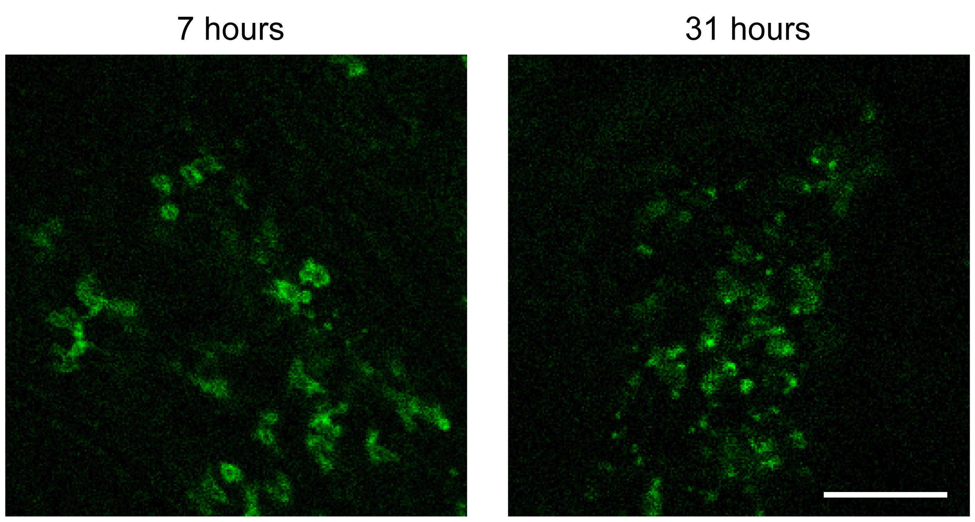
      Figure 1. Effect of varying antibody penetration times. Seven hours after RO injection of CD8α antibody (left), intestinal intraepithelial lymphocytes (IEL) show a classic membrane staining pattern. In contrast, 31 h after injection (right), IEL have internalized the CD8α antibody, leading to smaller, punctate signals. Scale bar = 100 μm. Brightness of each image was adjusted independently, and a green lookup table was used to improve visibility of the features.

      
      

   2. If you are only using one antibody, we recommend choosing a far-red fluorophore (e.g., Alexa Fluor 647) due to that channel’s lower autofluorescent background. For the two-channel imaging used here, we also used a green fluorophore (Alexa Fluor 488) to minimize channel bleed through.

      Use IgG antibodies directly conjugated to organic dyes, such as Alexa Fluor 488, 555, or 647. Avoid antibodies conjugated to bulky fluorescent proteins (such as phycoerythrin or allophycocyanin), as their large molecular weight impedes efficient diffusion into tissues and, while they are initially bright, they bleach quickly.

   3. Dilute 15–20 μg of antibody (here, anti-CD8α and/or anti-EpCAM antibody) in 50 μL of sterile PBS.

   4. Anesthetize the mouse with isoflurane and inject the antibody solution retroorbitally (Yardeni et al., 2011) It is important to inject the full volume of labeled antibody for consistent labeling without introducing any air bubbles in the mouse’s circulation.

   5. Return mice to cages for recovery. Mice need to be fasted for 4 h to slow down peristalsis.

      
      

2. Suction ring setup

   1. Suction rings, originally developed for lung imaging (Looney et al., 2011), offer a convenient way of stabilizing many mouse tissues. The rings we used were custom made at a CNC machine shop (see Notes for recommended supplier). An alternative design utilizes a resin 3D printer (Ahl et al., 2019) and contains an embedded electrical heater to provide more physiological thermal conditions during imaging. Ahl et al. (2019) provides an elegant description of the complete vacuum system and includes the 3D stereolithography [files for the 3D printer (in .stl format)]. An alternative device, which uses clamping instead of vacuum pressure, is described in Koike et al. (2021).

   2. In this protocol, we based our part selection on United States American National Standard Pipe Thread (NPT). In this standard, fittings are based in inches. According to the standard, 3/8” barbed fitting will have a good fit for a 3/8” (9–10 mm) internal diameter vacuum tubing. The barb diameter is slightly larger than the tubing diameter to ensure a proper seal. You can modify the design to use materials available in your country or already existing in your laboratory. For the best performance of the vacuum system, you should try to maximize the internal diameter of the parts, minimize the total length of the circuit, and eliminate all leaks. Online suppliers such as Amazon, Fittings, Inc., or US Plastic Corporation offer a convenient source of parts. A local hardware or automotive stores can also serve as valuable resources for users who need additional help in procuring the parts or assembling the circuit.

   3. Assemble the vacuum system (Figure 2). The suction ring is connected to a small vacuum trap to collect any biological fluids. From there, it is connected to a fine adjustment valve, a coarse adjustment valve, and a gauge to read the vacuum pressure. Finally, it is connected to the central building vacuum through a filter as a secondary method to prevent any contamination. Connect the pieces in the following order:

      1. Connect the hydrophobic filter disk to the central vacuum shutoff valve with the 3/8” thick-walled vacuum tubing.

      2. Attach the tubing to the barb of the 1/4” NPT female connector, and couple it to a male-male coarse adjustment valve using Teflon tape.

      3. Couple the NPT connector with the female Tee connector.

      4. Add the male-male extension nipple to the top of the Tee connector and fit the pressure gauge on top with the female-female 1/4” NPT coupling.

      5. Attach the 1/4” NPT male to 5/16” barb connector to the Tee connector and fit the 5/16” vacuum tubing.

      6. Add the plastic T-splitter and attach the 2-way stopcock fine adjustment valve on a length of tubing that will allow placement of the stopcock within reach of the surgeon. This valve can be opened to reduce the vacuum or closed to increase it. An alternative design can use an aquarium pump valve.

      7. Attach the small vacuum trap with 5/16” vacuum tubing and secure it upright.

      8. Add required length of the vacuum tubing to reach the microscope and connect the 1/4” barb to Luer lock connector. Add Teflon tape if needed to ensure proper seal.

         
         

      
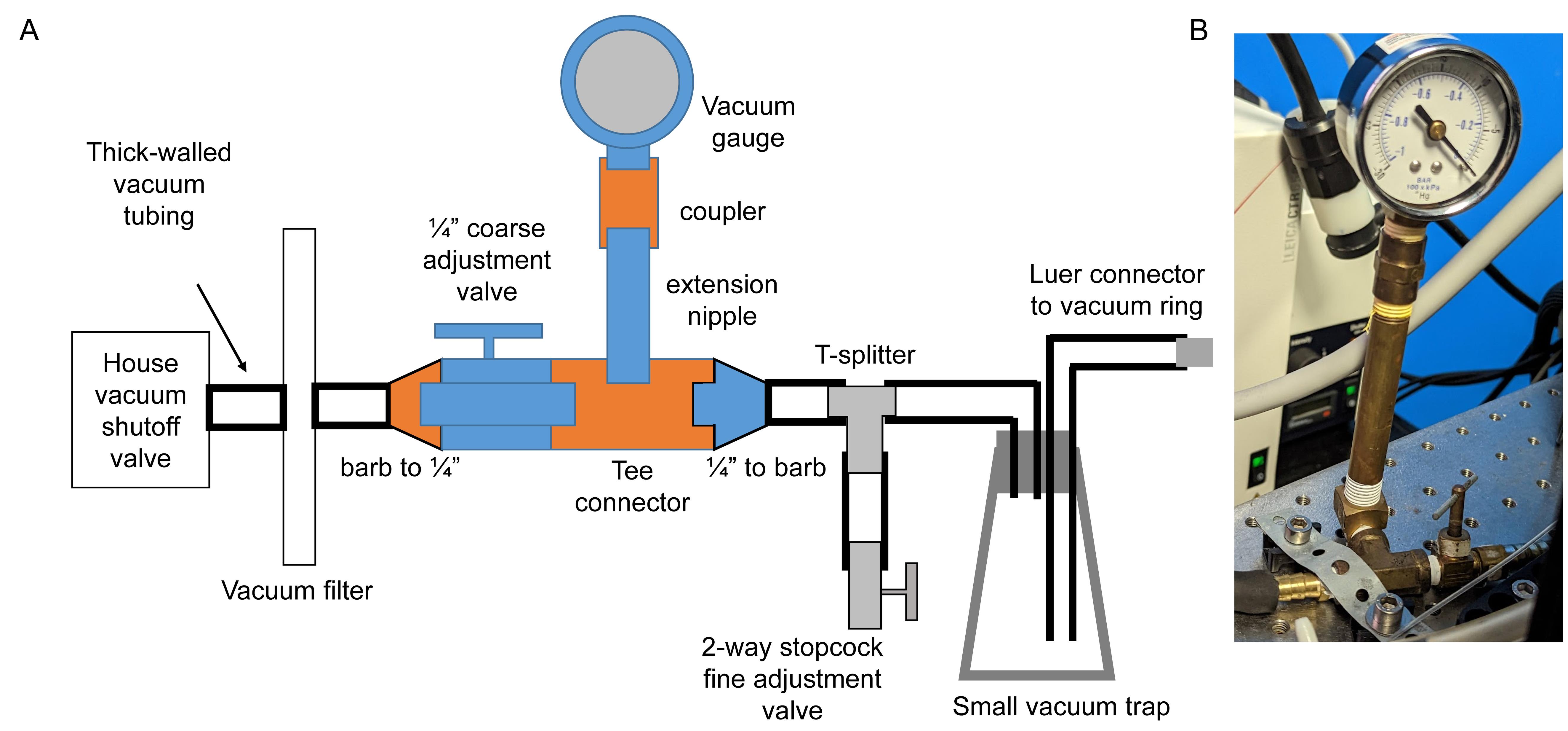
      Figure 2. Schematics of vacuum circuit. A. Parts with female NPT connectors are indicated in orange; parts with male NPT connectors are indicated in blue. Grey parts are plastic luer-type or barbed connectors. B. Example build with vacuum gauge and adjacent parts.

      
      

   4. Remove the plunger from a 10 mL syringe and squeeze a large bead of the vacuum grease into the syringe. Insert the plunger and apply a thin line of grease on the edge of the ring. Use Dumont #5/45 forceps to distribute the grease evenly on the rim of the ring. Remove any grease that got into the groove of the ring.

   5. Clean a #1.5 12 mm diameter coverslip with 70% alcohol and wipe on lens paper to remove any traces of dust and lint. Place the coverslip on ring and press down to seal (Figure 3A).

   6. Place the suction ring assembly on a post raised above the microscope stage and secure it with a right-angle post clamp or swivel clamp. We use a custom-made aluminum block with the post attached, screwed into the microscope stage for maximum stability, which can be requested at a machine shop. Make sure the cover glass is perpendicular to the optical axis of the microscope by aligning the ring parallel to the lens of the objective (Figure 3B).

      
      

      
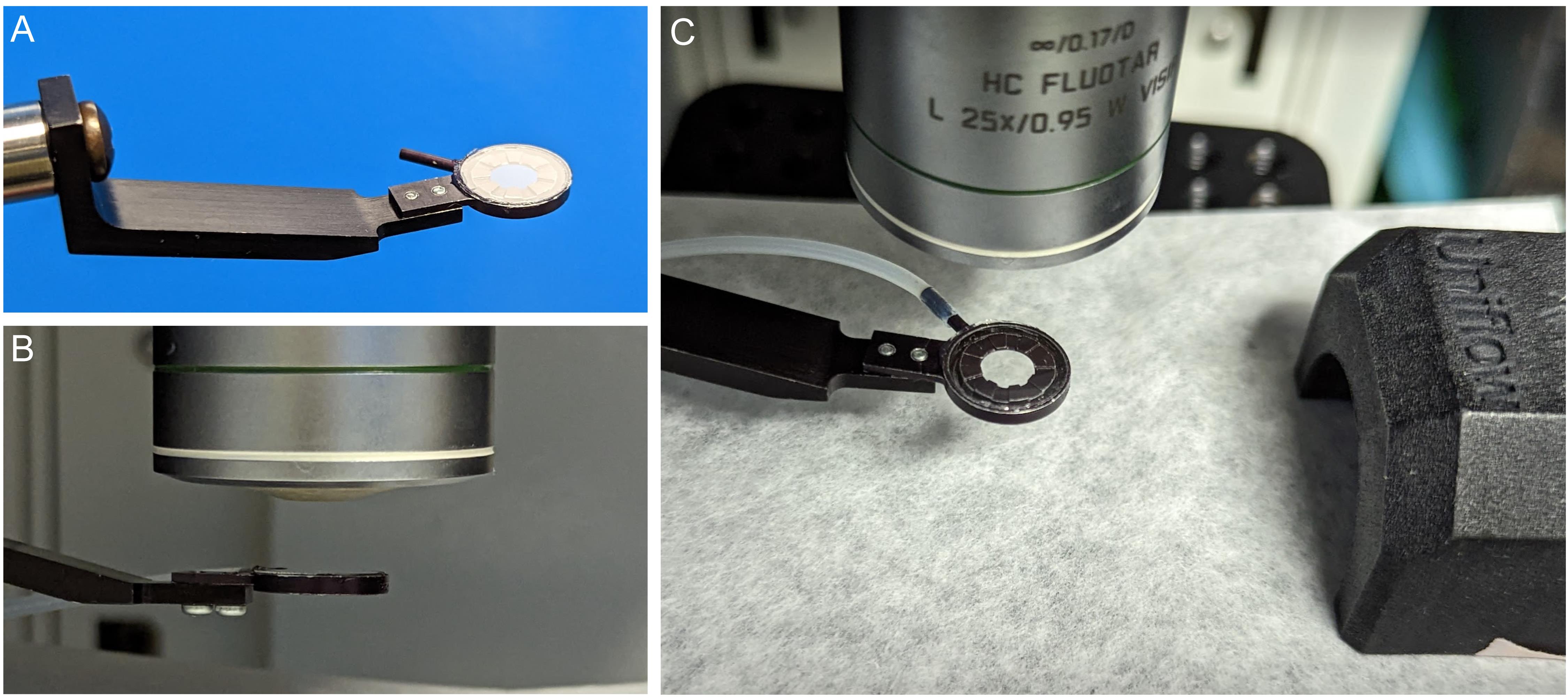
      Figure 3. Assembling the suction ring. A. Attach a #1.5 coverslip to suction ring with vacuum grease and attach PE160 tubing. B. Adjust the ring to be parallel to the front lens of the objective. C. Position the suction ring and the nose cone on the heated platform.

      
      

   7. Connect the suction ring via 18 G blunted needle end to the Luer lock of the vacuum circuit. Set the system to 5–20 mbar vacuum pressure. The exact value is dependent on the preparation and the way in which the system is integrated. Use the lowest vacuum pressure sufficient to stabilize the tissue.

      
      

3. Microscope setup

   1. Insert the objective onto the piezo Z controller.

   2. Open the acquisition software and initialize the resonant scanner.

   3. Turn on appropriate laser lines and initially set the power to a low setting (~5%). In our case, we imaged using the 488 and 638 nm lines.

   4. Select a dichroic filter that will give you the ability to switch between laser lines without needing to move any hardware. In our case, it was the 488/552/638 triple dichroic mirror for the SP8 system. For optimal use of confocal reflection microscopy for label-free detection of tissue structure, use the Reflection/Transmission mirror.

   5. Set up the internal detector wavelengths, assigning the fluorescence gathered from antibody labeling on your most sensitive detectors (in our case, HyD detectors). These wavelengths were selected for AF488, AF647, and the confocal reflection channel:

      1. AF488: 494–563 nm

      2. Reflection: 619–651 nm

      3. AF647: 651–722 nm

   6. Either the tissue reflection or EpCAM staining for epithelium can be used to identify SI anatomy, although they provide slightly different information (Figure 4).

      
      

      
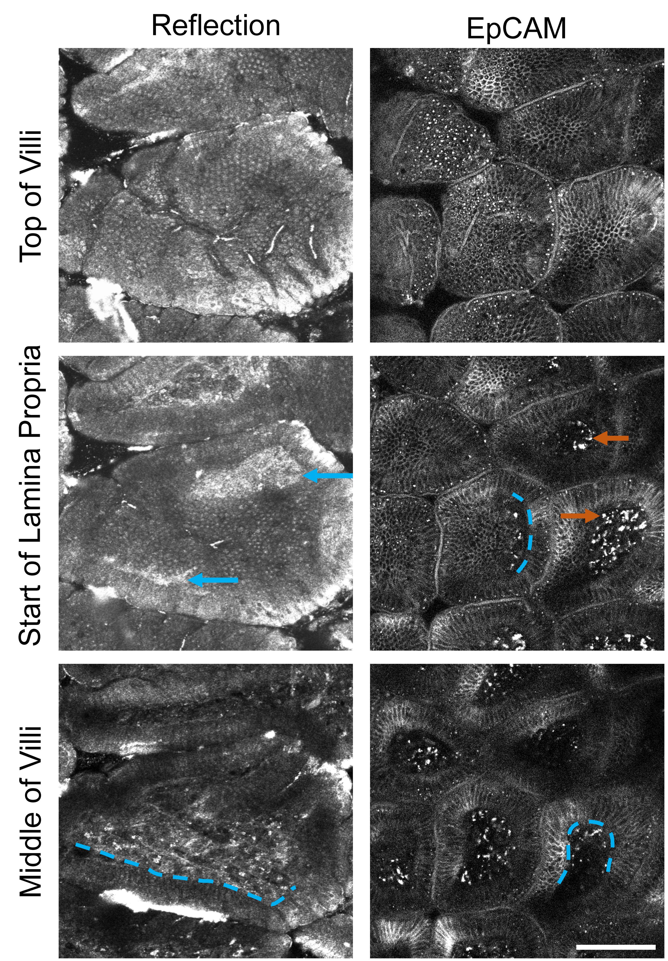
      Figure 4. Comparison of visible structures from tissue reflection (left) and EpCAM staining (right) at three depths through the small intestinal (SI) villi. Brightness is adjusted in each image individually to accent details. Scale bar = 100 μm. Blue dotted lines = location of basal lamina. Blue arrows = basal lamina visible by reflection microscopy. Orange arrows = autofluorescent debris or non-specific binding of EpCAM antibody to macrophages.

      
      

   7. Set the system to perform XYZT imaging, with the Z stepper controlled by the piezo element.

   8. Adjust the pinhole size to two Airy units, enable bidirectional scanning, and find the appropriate phase correction. Enable line averaging during live acquisition setting and set the data acquisition mode to 8-bit. Set the zoom to the minimum allowed by the system for biggest field of view and adjust the line averaging to at least 8×. Our pixel size was set to approximately 0.6 μm with a corresponding field of view of approximately 370 μm.

      
      

4. Surgery and intravital microscopy

   1. Please ensure all mouse handling and surgery steps are written in your Animal Care Committee–approved protocol. The following procedure is rather complex, with the scientist needing to simultaneously pay attention to the mouse anesthesia, the vacuum window pressure, and the image acquisition. We highly recommend practicing each part of the procedure slowly before attempting the full intravital imaging workflow. For example, a novice user can test the labeling, vacuum window, and image acquisition by practicing with a mouse that has been euthanized 4 h after antibody injection.

   2. We found that preparations with isoflurane alone had too much movement (Video 1). Ketamine/xylazine anesthesia followed by isoflurane inhalation creates the best conditions for imaging with reduced motion artifacts (Figure 5, Video 2). Prepare the ketamine/xylazine mixture in sterile PBS (10 mg/mL ketamine and 1.5 mg/mL xylazine). Weigh the mouse and deliver 10 μL of the prepared solution per gram of body weight (100 μg of ketamine and 15 μg of xylazine per gram of mouse weight) via intraperitoneal injection.

      
      

      
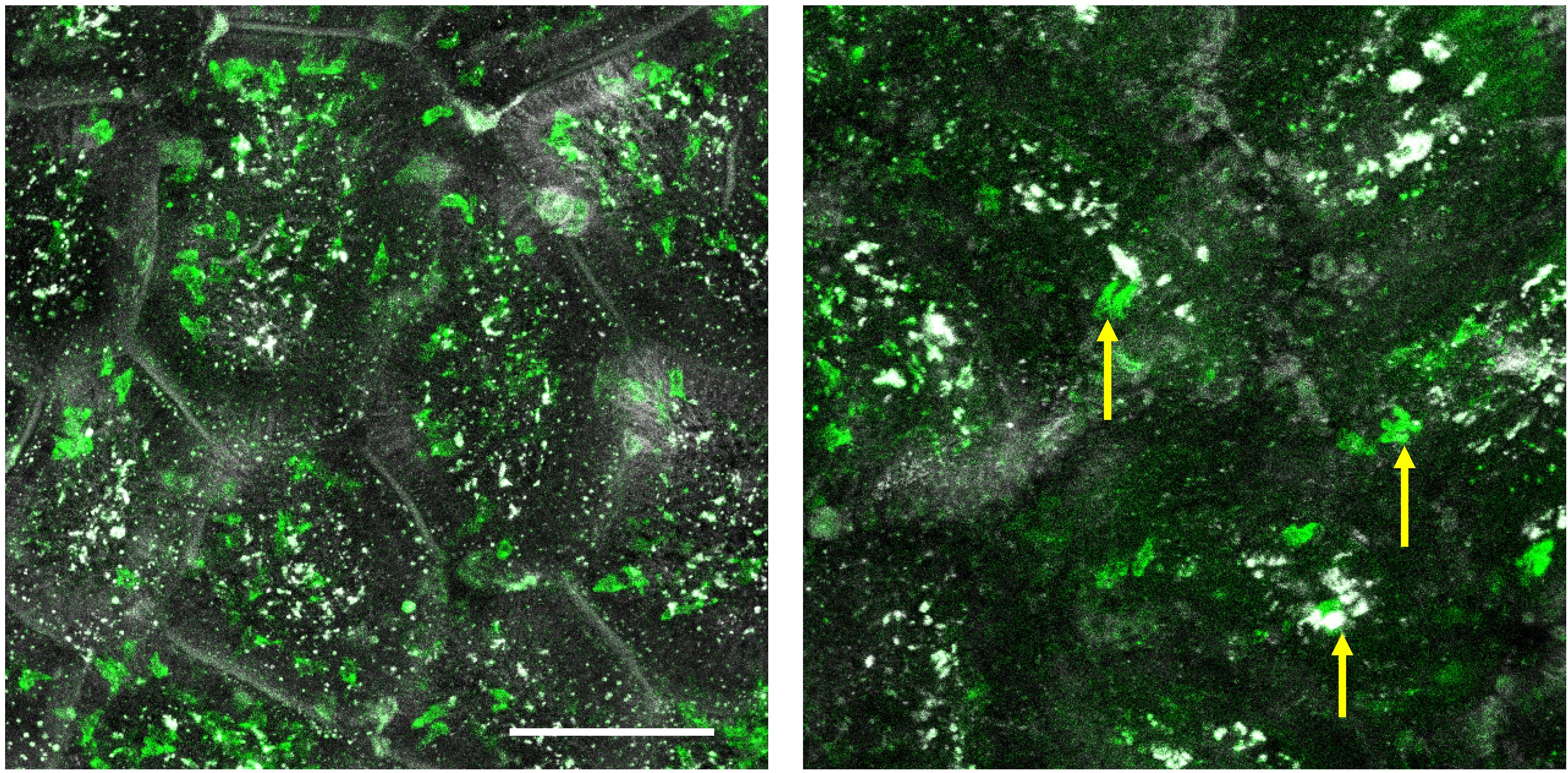
      Figure 5. Example images from a well stabilized (left) and poorly stabilized (right) intravital movie. The image on the left was taken using a mouse anesthetized with both ketamine/xylazine and isoflurane; the image on the right was from a mouse anesthetized only with isoflurane. These are Z projections of single time points. Yellow arrows point to cell shadows that are caused by significant tissue motion between sequential Z steps, compromising the accuracy of the analysis. Green = CD8α; White = EpCAM. See also supplementary movies. Brightness was adjusted in each image. Scale bar = 100 μm.

      
      
      
      Video 1. Representative movie from an insufficiently stabilized preparation (isoflurane-only) that cannot be accurately quantified. Maximum intensity Z projection of a 10 min time series. Green = CD8α; White = EpCAM. Scale bar = 74 μm. See also Figure 5.

      
      

      
      Video 2. Representative example of a well stabilized movie from a mouse anesthetized with isoflurane and ketamine/xylazine. Maximum intensity Z projection of a 10 min time series. Green = CD8α; White = EpCAM. Scale bar = 74 μm. See also Figure 5.

      
      

   3. After anesthesia onset, shave the abdominal area with clippers or with hair removal lotion, followed by cleaning with 70% isopropanol.

   4. Place the mouse ventral side up on heating pad and place the snout of the animal in isoflurane facemask. We place a thin steel plate over the ATC2000 heating pad, connected with thermal paste, to enable the use of a magnetic isoflurane mask. Alternatively, you can tape the isoflurane mask directly onto the heating pad.

   5. Turn on isoflurane flow to face mask. Observe the breathing pattern of the animal and maintain a stable plane of anesthesia by delivering between 0.5% and 2% isoflurane. Labored breathing indicates the animal has been anesthetized too deeply.

   6. Secure the limbs of the mouse with laboratory tape.

   7. Insert a Vaseline-coated rectal thermometer and secure it by taping it to the tail. Set the feedback loop of the animal temperature controller to 37 °C.

   8. Verify that a sufficient anesthesia level has been reached with a toe pinch (Figure 6A).

   9. Position the ring assembly above the center of the abdomen and adjust it such that it is parallel to the front lens of the objective (Figures 3B and 6H). You might need to reposition the mouse to ensure that the ring has unobstructed access to the area. It is much safer to reposition the intact animal before incisions. Move the ring out of the way for surgery.

   10. Make an approximately 2 cm midline incision in the skin with surgical scissors (Figure 6B). Locate the linea alba and make a 1.5 cm incision along it in the peritoneum to expose the small intestine, taking care to avoid inadvertently introducing hair in the surgical area or cutting through blood vessels (Figure 6C).

   11. Using two wetted cotton tipped applicators, delicately move the intestine and position the antimesenteric side upwards. Look for areas that are free of food matter. Take care not to accidentally twist the gut and pinch the blood supply. Locate the stomach and find the piece of intestine distal to it. This will be the distal duodenum or jejunum. Exteriorize a small loop through the opening in the peritoneum (Figure 6D). Notice the blood vessels on both sides of the intestine and avoid cutting or damaging them. Using a cautery set to medium power, gently cauterize the antimesenteric surface of the intestine (Figure 6E). With small scissors, make an approximately 1 cm long opening along the cauterized edge (Figure 6F). Use cotton tipped applicators to gently open and flatten the gut, revealing the mucosal surface of the villi (Figure 6G). You may also use forceps but grab only the edges of the tissue.

       1. Work quickly to avoid drying the tissue. If necessary, you can add a drop of PBS onto the mucosal surface to keep it moist. However, it is best not to disturb the mucus layer over the villi, because this will increase the amount of tissue movement.

       2. If you notice any bleeding, cauterize the wounded area immediately. If excess blood has pooled near the region of interest, add a drop of PBS and use gauze or a cotton tipped applicator to remove the excess. It is important to minimize blood loss because any blood on the imaged area will reduce the fluorescence intensity, but, as above, washing the tissue can damage the mucus and cause additional tissue motion.

   12. Hold the suction ring in your dominant hand and lower it onto the exposed mucosal surface. Control the waste vacuum valve with your other hand and adjust the pressure to the lowest possible setting that achieves a complete seal against the tissue. You should see that the tissue is flattened against the coverslip (Figure 6H). Because the required pressure depends on how well the intestine seals to the ring, it is less important to keep the measured pressure consistent than ensuring the tissue is stable and undamaged in each preparation.

       
       

       
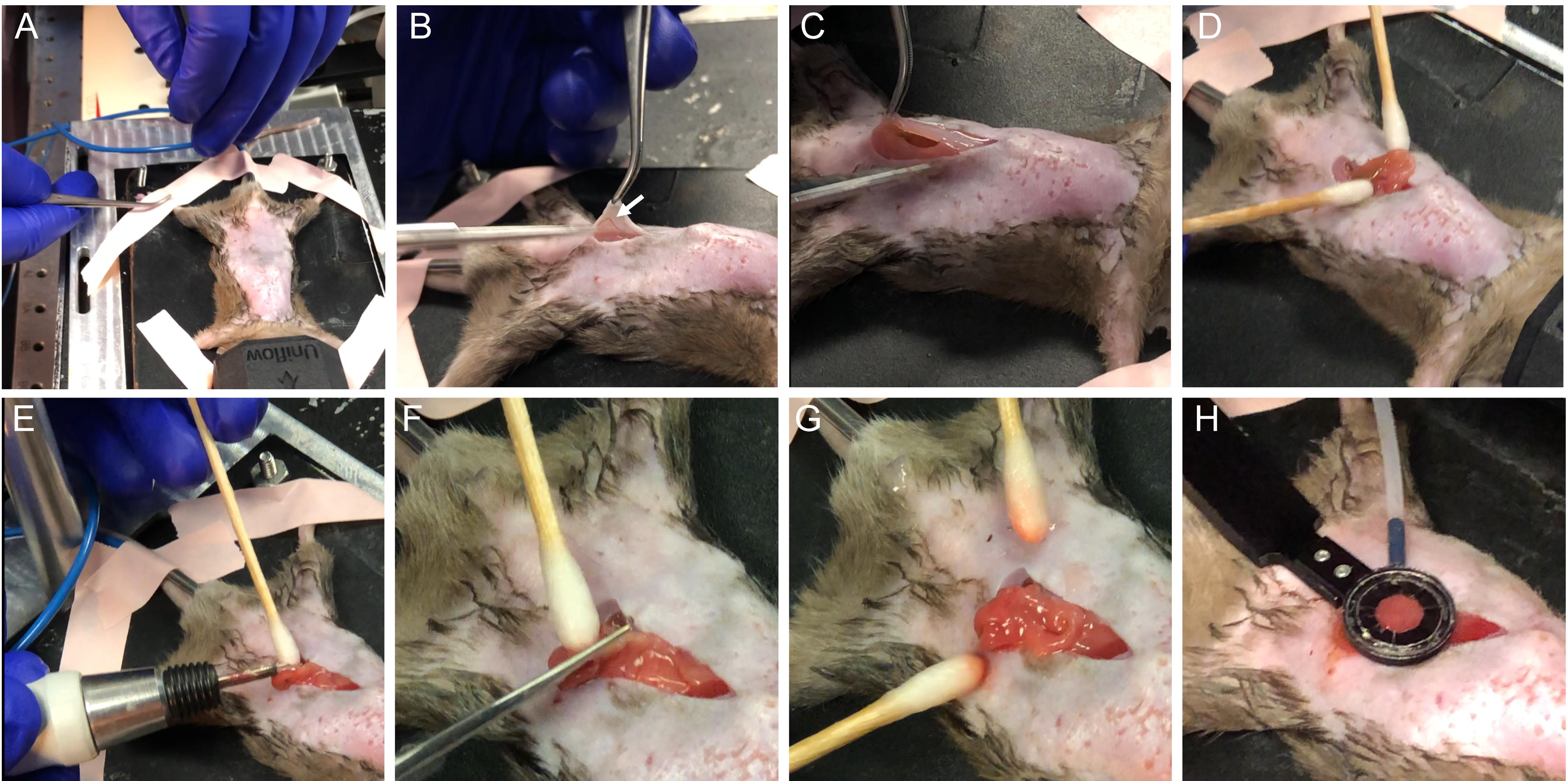
       Figure 6. Overview of the surgical procedure. (A) Secure the animal and verify adequate anesthesia. (B) Make a midline incision taking care not to damage skin blood vessels (arrow). (C) Open peritoneum along linea alba and avoid major vessels. (D) Gently exteriorize the gut and find appropriate section free of food. (E) Cauterize the antimesenteric side. (F) Cut along the cauterized area to open the intestine. (G) Gently stretch and flatten mucosal surface. (H) Position suction ring above the exposed intestine and gently lower it onto the tissue while adjusting suction force to adhere the tissue to the coverslip.

       
       

   13. Add a drop of PBS on top of the coverslip for immersion and lower your objective to make contact with the fluid. With a long working distance objective, you will typically need to move the objective away from the ring to find the focus.

   14. Using the 25× (0.95) objective and a green fluorescence filter cube, look through the eyepiece and observe the preparation under epifluorescence illumination. Erythrocytes in capillaries of the villi should be traveling at a high speed; you might see an occasional bigger immune cell moving through the blood stream. If the tissue is moving, gradually increase the pressure with the fine adjustment. Alternatively, inspect other areas within the vacuum ring to find a more stable location. You can further increase the stability of the preparation by gently lifting the ring by a few millimeters to isolate the attached tissue from the mouse’s respiration (Move the objective out of the way before attempting this.). If you can see erythrocytes stopped in capillaries or moving in a backwards and forward motion, your vacuum pressure is too high, or you raised the preparation too much and the blood vessels have become pinched. Good preparations should show minimal movement of the villi and robust perfusion through the capillaries.

   15. Start image acquisition in live mode and adjust the gain and laser power as necessary to utilize the full dynamic range without saturation. Image in simultaneous mode after calibrating the detectors’ gains and wavelengths to avoid bleed through. Choosing optimal parameters for intravital imaging involves balancing the need for high acquisition speed to track moving cells, high sensitivity to detect dimly labeled cells, and large field-of-view to make the most of every labor-intensive experiment. For more details on acquisition setup for intravital imaging, please see the review (McArdle et al., 2016).

   16. Set the top and bottom of Z stack to encompass the top of the villus, the subepithelial area, and lamina propria. The basal lamina can be seen by reflection microscopy (Figure 4, blue arrows). If you use EpCAM labeling, the transition between the epithelium and lamina propria is visible as a distinct change in tissue texture (Figure 4, blue dotted lines showing some examples). Autofluorescent or non-specifically labeled macrophages are characteristic cells in the lamina propria that serve as a useful landmark (Figure 4, orange arrows).

   17. Adjust the step size to 2.8 μm. Set the timelapse imaging to acquire Z stack every 30 s or faster, trimming the Z stack if needed. Acquire data for a minimum of 10 min per location. Save the data as .lif file.

   18. Monitor the mouse plane of anesthesia throughout the experiment by observing the breathing pattern every 5–10 min and adjusting the amount of vaporized isoflurane as needed. Do a pinch test between the acquisitions to verify if the animal is fully anesthetized.

   19. After completion of the imaging, euthanize the animal according to your approved protocol.

   20. Clean the ring with PBS and 70% alcohol and remove the coverslip and any remaining vacuum grease.

       
       

5. Image processing

   1. The suction ring often provides enough stability to the tissue to proceed with analysis without further motion removal. However, if necessary, small motion artifacts can be minimized after acquisition in Fiji (Schindelin et al., 2012). Whether the mechanical stabilization is sufficient for cell tracking is determined visually. Loosely, post-processing is necessary if there was gross tissue motion between Z steps or between sequential time steps of > 1/2 of a typical cell diameter (Figure 5).

      1. Open the 1–3 channel .lif file in Fiji as a hyperstack using the Bioformats importer. Delete any Z steps that are entirely outside of the detectable tissue or region of interest because blank images without meaningful signal disrupt the alignment algorithm.

      2. Change the color of each channel to either red, green, or blue, and then flatten the multichannel image to an RGB image. (This step can be skipped if there is only one channel.)

      3. If each villus shows independent motion that ought to be corrected separately, create small crops of each villus. Each cropped region should be just large enough to capture the entire villus through all Z stacks and time points. Process all further steps independently for each region.

      4. Apply the MSTHyperStackReg2 plugin (Ray et al., 2016). This software first aligns each Z step of each time point individually. Next, a maximum intensity Z projection is created to register the time series, and the calculated transform for each time step is applied to each Z position. At each stage, the entire sequence (either in Z or in T) is registered using minimum weighted spanning trees to choose a reference image and to ensure that outliers (images with particularly extreme motion artifacts) do not degrade the quality of the global alignment. This algorithm corrects lateral tissue movement in X and Y but does not correct vertical drift (Z motion).

         i. First, perform coarse registration. We recommend using rigid body alignment using the approximate with a large graph width (the larger of half the number of Z steps per stack or half the number of time points) and allowing it to automatically choose the anchor image and add a border (Figure 7A). The automatically produced maximum intensity image can be used to visually check the alignment. Save the aligned Z stack as an intermediate step. High quality images with small non-linear tissue distortions can be successfully corrected using affine transformations, though affine transforms often produce very bad results from noisy or sparse images.

         ii. Next, perform fine alignment on the results. We recommend using rigid body transforms, the exact method, a small (i.e., 5) graph width, automatic anchor selection, and no additional border (Figure 7A). This step can take a long time (hours), depending on the dimensions of your image and the graph width.

         iii. The improvement in image quality using image registration is illustrated in Video 3 by comparison to Video 2.

         
         
         
         Video 3. Improvement in image quality using image registration. The 3D data from Supplementary Video 2 was processed with MISTICA image alignment, which minimized jitter and drift. Maximum intensity Z projection of a 10 min time series. Green = CD8α; White = EpCAM. Scale bar = 74 μm.

         
         

      5. In Fiji, adjust the image properties to set the voxel dimension and time step. Save the final result as a .tif hyperstack.

   2. Immune surveillance of the epithelium can be measured by calculating the area covered by all labeled cells during a set amount of time in Fiji.

      1. Load the raw .lif file or the aligned .tif hyperstack into Fiji.

      2. Use the reflection signal or the EpCAM channel to identify the epithelial layer. At the top of each finger-like villus, there is a region approximately 10 μm deep that is nearly exclusively epithelium. IEL often migrate along the basement membrane separating the SI epithelium from the lamina propria. Create a substack of the volume encompassing the epithelium at the top of the villus and the basement membrane and trim each video to a set amount of time (e.g., 10 min).

      3. Using the polygon tool, draw a region of interest (ROI) encircling each villus and save each region to the ROI manager (Figure 7B).

      4. Split the channels. On the CD8α channel, use a median filter (2D, radius 2 pixels) to remove pixel noise.

      5. Create a maximum intensity Z projection and then a maximum intensity T projection to combine all timepoints and Z locations into a single image, which has the location of every cell overlaid in the 10 min movie (Figure 7B).

      6. Using the threshold tool, determine the intensity threshold that separates cells from background non-specific signal (Figure 7B). Ideally, this can be determined by performing one preliminary experiment with a labeled isotype control antibody. In the absence of this negative control sample, set the threshold to be just under the intensity of the dimmest labeled IEL. Use the same threshold for all samples by pressing the Set button and typing the determined threshold. Apply the threshold to binarize the image.

      7. In Fiji, set the measurements to include area and area fraction; uncheck limit to threshold. Measure each ROI defining a villus. The results window will report the total area of the villus and the fraction that was visited by a cell in the time period (Figure 7C).

      8. The movement of the cells can be displayed with a rainbow time projection (Figure 7D). Use the maximum intensity Z projection time series from step 2e and apply the Fiji plugin Temporal-Color Code (Miura, 2022) to show each time step as a unique color. Fast cells will appear as rainbow streaks while immobile cells appear white (all colors overlaid).

         
         

         
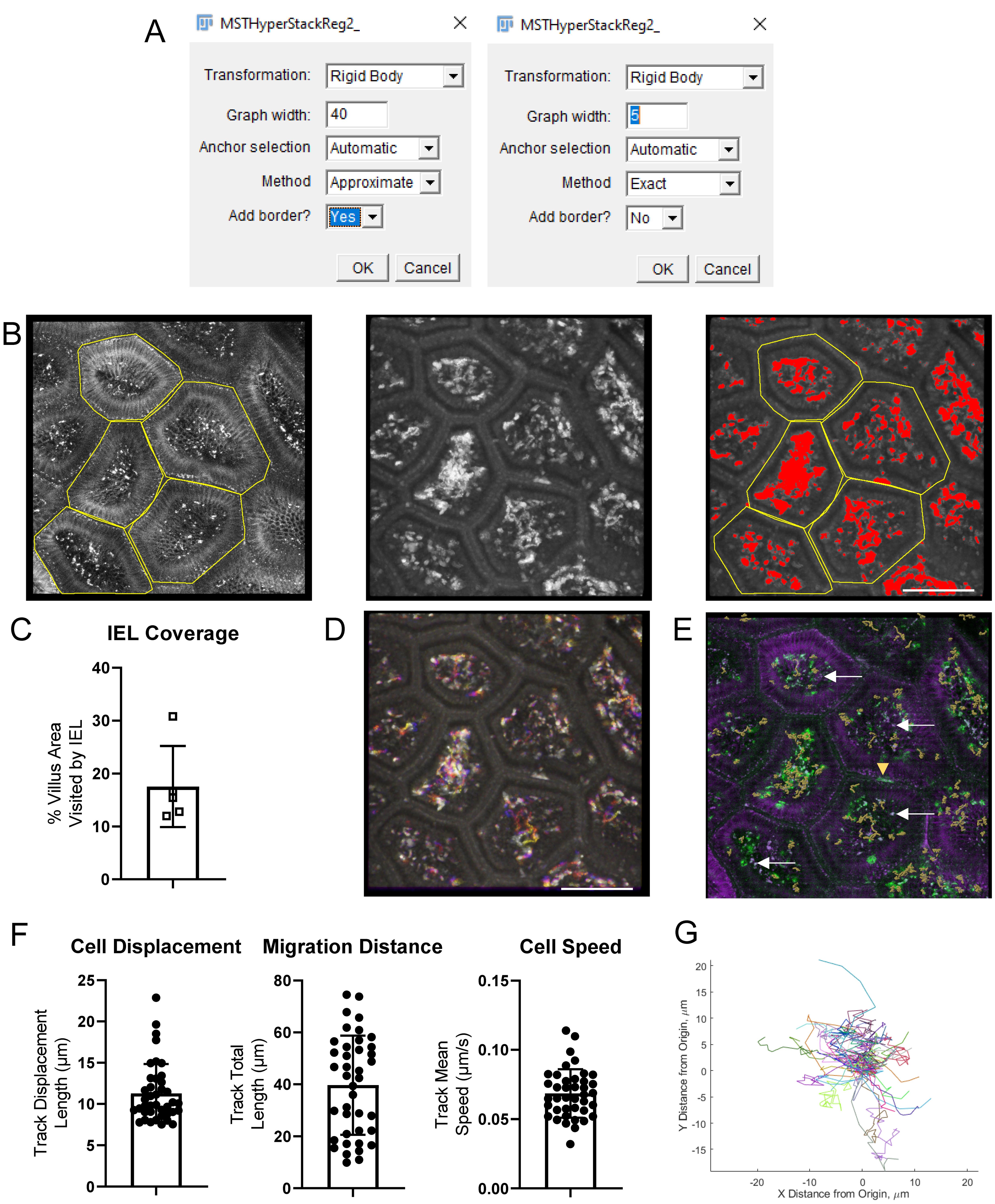
         Figure 7. Examples of image processing steps and results. A. Screenshots of MSTHyperStackReg plugin parameters for an image with 85 Z-steps and 40 timepoints. Left: First round (approximate) settings, with graph width half of the Z stack. Right: second, more precise round of alignment. B. Screenshots of intermediate results during the calculation of villi coverage by intestinal intraepithelial lymphocytes (IEL). Left: Each villus is outlined using the EpCAM channel. Middle: median smoothing is applied to the CD8α channel and a maximum intensity projection over all Z steps and all time points is applied to overlay the position of every IEL. Right: a threshold is applied to find the area visited by an IEL at least once during the 10 min movie and the villi outlines are overlaid (yellow). C. In each villus, the percentage of the area visited by an IEL is calculated. D. Alternatively, IEL movement can be displayed as a rainbow time projection. E. CD8α-AF488 IEL (green) were tracked in Imaris. The tracks are shown as orange lines. EpCAM-AF647 (purple) marks the small intestinal (SI) epithelium. White arrows show a few of the many examples of artifacts that are visible in both the AF488 and AF647 channels. The yellow arrow shows a non-specifically labeled cell. F. Cell displacement, total movement distance, and speed were calculated from the Imaris tracks. G. The migration of each cell is shown as a spider plot. Scale bars = 100 μm.

         
         

   3. Movement statistics, such as mean speed, track length, and displacement demonstrate cell activation and patrolling behavior. Track the IEL in 3D in Imaris to quantify cell motility.

      1. In Imaris, open the raw .lif files or tifs aligned in Fiji. If you are working with processed tifs, it is a good idea to check the voxel size and time step information in Image Properties.

      2. If necessary, correct slow lateral and axial drift affecting the entire imaged volume in Imaris before cell tracking.

         i. Use the Spots function to track bright, stable features, such as immobile cells, or autofluorescent or reflective debris. Please see below (step 3c) for details on the Spots function. Choose 3–10 spots that span the entire volume under analysis for the entire time series.

         ii. In the Edit Tracks tab, select Correct Drift. Choose the options for correcting the image and objects, using translational and rotational drift, and include the entire result.

      3. Tracking the movement of IEL can be performed semi-automatically with the Spots wizard (Figure 7E). The exact parameters need to be optimized for each project, but the overall process is similar in all cases. Detect round objects in your chosen channel (CD8α) and then apply quality, size, and intensity filters to remove debris and macrophages that have picked up the antibody. The most sensitive parameter is usually the expected object diameter; be sure to choose the typical diameter of the fluorescent spot, which may be smaller than the cell diameter if the antibodies have been internalized or if the cells are polarized. Add object filters to remove debris that is bright in multiple channels. Imaris then performs tracking of the segmented objects over time. For well-stabilized movies, the autoregressive motion algorithm usually produces the best results, although the Brownian motion algorithm can work in some cases. At this stage, adding track filters to remove stationary objects can improve performance.

      4. There will nearly always be mistakes in the automatic tracking for intravital imaging data: single tracks inappropriately split, tracks jumping between neighboring cells, or non-IEL objects being included. Surface-labeled IEL can be distinguished from other objects by their shape (hollow, round), speed (greater than local tissue motion), and directionality (movement along basal lamina, as opposed to transverse). If multiple channels were imaged, autofluorescent objects can be seen in all channels, whereas antibody signals are usually much brighter in the proper channel (Figure 7E). Correct the centroid spots and connecting tracks manually in the Edit tab of the Spots object. It is important to use the same level of care and attention on all samples; manually correcting some images but not others can bias the final results. For further information on how to perform tracking in Imaris, please refer to Bitplane’s extensive online tutorial library.

      5. In the Statistics tab, export the track speed, track length, and track displacement metrics to a csv file. (Figure 7F). Use the export data for plotting to export the cell positions at each time point in a convenient three-column format.

      6. Spider graphs are an informative way to visualize cell migration. In these graphs, each cell starts at position (0, 0) and its total path is drawn in a random color, demonstrating overall cell motility and directionality.

         i. The spider plots can be generated from the exported cell position data using a simple script or stand-alone application found on GitHub (github.com/saramcardle/IEL) (Figure 7G).

         ii. Alternatively, a spider graph can be generated in Imaris. First, select all the IEL tracks and duplicate the spots. In the new spots object, select all of the tracks and then apply the Translate tracks function in the Tools tab. This will move all of the tracks to originate at the same location. The newly adjusted position of each cell can be exported to a spreadsheet for plotting.

   4. Limitations of image analysis

      1. The cell-by-cell statistics produced here inherently have high variance due to natural biological variability (see plots in Figure 7). Additionally, each experiment only yields a small number of tracked cells (~20–40). Therefore, it is only possible to detect large differences between groups.

      2. Even with tissue stabilization and drift correction, some tissue movement is usually still present. This tissue movement defines the lower limit of reliable quantification for cell speed and travel distance. To measure this for each dataset, track some autofluorescent spots that should not move during image acquisition, such as macrophages and food debris, using the Imaris spots wizard. Calculate their average speed and travel distance. The results show the sensitivity of your measurements; differences between cell groups smaller than typical gross tissue movement should be ignored, and preparations with unusually large tissue movement should be discarded.

      3. Sometimes, it can be difficult to distinguish antibody-labeled IEL from non-specific signals or autofluorescent objects. It is important to optimize the antibody concentration and injection time for your specific experimental protocol. Additionally, it can be helpful to perform a preliminary experiment using an isotype control antibody to visualize the intensity, location, and shape of artifacts as a negative control.

      4. Please plan your experiments to minimize batch effects. If comparing two (or more) groups of mice, always image a mouse from each group back-to-back using the same batch of antibodies. Alternate which group is chosen to be run first each day, so that there is no systemic bias in the length of antibody incubation time or fasting time.

         i. For projects comparing the activity of different cell populations, rather than different mouse conditions, it is possible to image two cell populations simultaneously with two different fluorophore-labeled antibodies. In this case, the movement characteristics of one population can be normalized to that of the other population in each mouse individually. This is an elegant way to minimize the differences in tissue motion in each preparation.

Notes

It is vital to consult your Institutional Animal Care Committee or equivalent body to ensure that all procedures were reviewed and approved according to the governing laws.

Intravital microscopy is a complex procedure. As each microscopy system is unique, it is best to seek advice from core facility staff or experienced users on how to establish the best parameters for imaging. Novice users should first master the handing of the microscope using an immobile object, such as a euthanized mouse injected with an antibody targeting the cells of interest. We encourage using untreated littermate control animals to understand the nature of autofluorescence in the tissue. Animals that received isotype control antibodies can serve as valuable controls for the specificity of antibodies targeting cells of interest. By comparing the images obtained from these kinds of samples, novice users can develop understanding of proper labeling and learn to distinguish it from artifacts and autofluorescence, which is often very strong in the lamina propria. For additional information on intravital microscopy in the gut, we refer readers to previous studies by Sujino et al. (2016), Chen et al. (2019), and Koike et al. (2021).

The suction ring assembly can be purchased from Zera Development Company; please see https://www.zeradevelopment.com for contact information. For the best performance of the vacuum circuit, make it as short as possible and seal all the leaks. Use Teflon tape to create a tight seal between metal parts of the system. Use large-bore vacuum tubing for connections between parts and minimize the volume of vacuum trap. Alternatively, the vacuum trap can be placed between the vacuum filter and the gauge assembly.

Acknowledgments

We wish to thank Dr. Grzegorz Chodaczek for sharing his expertise in intravital microscopy and for the development of suction ring techniques at La Jolla Institute for Immunology.

Funding: National Institutes of Health grants P01 DK46763, R01 AI61516, and MIST U01 AI125955 (MK); Chan-Zuckerberg Initiative Imaging Scientist Grant 2019‐198153 (SM).

This protocol is derived from the original research paper (Seo et al., 2022; DOI: 10.1126/sciimmunol.abm6931).

Competing interests

The authors have no conflicts or competing interests.

References

1. Ahl, D., Eriksson, O., Sedin, J., Seignez, C., Schwan, E., Kreuger, J., Christoffersson, G. and Phillipson, M. (2019). Turning Up the Heat: Local Temperature Control During in vivo Imaging of Immune Cells. Front Immunol 10: 2036.
2. Chen, Y., Koike, Y., Chi, L., Ahmed, A., Miyake, H., Li, B., Lee, C., Delgado-Olguin, P. and Pierro, A. (2019). Formula feeding and immature gut microcirculation promote intestinal hypoxia, leading to necrotizing enterocolitis. Dis Model Mech 12(12).
3. Cheroutre, H., Lambolez, F. and Mucida, D. (2011). The light and dark sides of intestinal intraepithelial lymphocytes. Nat Rev Immunol 11(7): 445-456.
4. Edelblum, K. L., Shen, L., Weber, C. R., Marchiando, A. M., Clay, B. S., Wang, Y., Prinz, I., Malissen, B., Sperling, A. I. and Turner, J. R. (2012). Dynamic migration of γδ intraepithelial lymphocytes requires occludin.Proc Nat Acad Sci U S A 109(18): 7097-7102.
5. Hoytema van Konijnenburg, D. P., Reis, B. S., Pedicord, V. A., Farache, J., Victora, G. D. and Mucida, D. (2017). Intestinal Epithelial and Intraepithelial T Cell Crosstalk Mediates a Dynamic Response to Infection. Cell 171(4): 783-794.e13.
6. Koike, Y., Li, B., Chen, Y., Ganji, N., Alganabi, M., Miyake, H., Lee, C., Hock, A., Wu, R., Uchida, K., et al. (2021). Live Intravital Intestine with Blood Flow Visualization in Neonatal Mice Using Two-photon Laser Scanning Microscopy. Bio Protoc 11(5): e3937.
7. Looney, M. R., Thornton, E. E., Sen, D., Lamm, W. J., Glenny, R. W. and Krummel, M. F. (2011). Stabilized imaging of immune surveillance in the mouse lung. Nat Methods 8(1): 91-96.
8. McArdle, S., Mikulski, Z. and Ley, K. (2016). Live cell imaging to understand monocyte, macrophage, and dendritic cell function in atherosclerosis. J Exp Med 213(7): 1117-1131.
9. Miura, K. (2022). Temporal-Color Coder plugin for Fiji. Shell. Fiji. Retrieved from https://github.com/fiji/fiji/blob/847ee410deedda9ba1de673820a5fa63446aa2e1/plugins/Scripts/Image/Hyperstacks/Temporal-Color_Code.ijm (Original work published 2011)
10. Mouse Room Conditions. (n.d.). The Jackson Laboratory. Retrieved November 19, 2022, from https://www.jax.org/jax-mice-and-services/customer-support/technical-support/breeding-and-husbandry-support/mouse-room-conditions
11. Ray, N., McArdle, S., Ley, K. and Acton, S. T. (2016). MISTICA: Minimum Spanning Tree-Based Coarse Image Alignment for Microscopy Image Sequences. IEEE J Biomed Health Inform 20(6): 1575-1584.
12. Schindelin, J., Arganda-Carreras, I., Frise, E., Kaynig, V., Longair, M., Pietzsch, T., Preibisch, S., Rueden, C., Saalfeld, S., Schmid, B., et al. (2012). Fiji: an open-source platform for biological-image analysis. Nat Methods 9(7): 676-682.
13. Seo, G.-Y., Shui, J.-W., Takahashi, D., Song, C., Wang, Q., Kim, K., Mikulski, Z., Chandra, S., Giles, D. A., Zahner, S., et al. (2018). LIGHT-HVEM Signaling in Innate Lymphoid Cell Subsets Protects Against Enteric Bacterial Infection. Cell Host Microbe 24(2): 249-260.e4.
14. Seo, G. Y., Takahashi, D., Wang, Q., Mikulski, Z., Chen, A., Chou, T. F., Marcovecchio, P., McArdle, S., Sethi, A., Shui, J. W., et al. (2022). Epithelial HVEM maintains intraepithelial T cell survival and contributes to host protection. Sci Immunol 7(73): eabm6931.
15. Sujino, T., London, M., Hoytema van Konijnenburg, D. P., Rendon, T., Buch, T., Silva, H. M., Lafaille, J. J., Reis, B. S. and Mucida, D. (2016). Tissue adaptation of regulatory and intraepithelial CD4⁺ T cells controls gut inflammation. Science 352(6293): 1581-1586.
16. Sumida, H., Lu, E., Chen, H., Yang, Q., Mackie, K. and Cyster, J. G. (2017). GPR55 regulates intraepithelial lymphocyte migration dynamics and susceptibility to intestinal damage. Sci Immunol 2(18): eaao1135.
17. Wang, X., Sumida, H. and Cyster, J. G. (2014). GPR18 is required for a normal CD8αα intestinal intraepithelial lymphocyte compartment. J Exp Med 211(12), 2351-2359.
18. Yardeni, T., Eckhaus, M., Morris, H. D., Huizing, M. and Hoogstraten-Miller, S. (2011). Retro-orbital injections in mice. Lab Anim (NY) 40(5): 155-160.
19. Zera Development Co. (n.d.). Zera development. Retrieved November 20, 2022, from https://www.zeradevelopment.com