Biophysical Analysis of Mechanical Signals in Immotile Cilia of Mouse Embryonic Nodes Using Advanced Microscopic Techniques

Materials and reagents

1. Coverslip (18 mm × 18 mm or 24 mm × 24 mm; No. 1S HT, Matsunami)

2. 400 μm silicone rubber spacer (discontinued product; alternatively, use AS ONE, catalog number: 6-9085-14)

3. 100 μm silicone rubber spacer (AS ONE, catalog number: 6-9085-12)

4. Rat serum (purchased from Charles River Laboratories Japan)

5. Fluorescent beads for Point Spread Function (PSF) measurement (Thermo Fisher, catalog number: F8811)

6. Polystyrene beads for optical tweezers (diameter 3.5 μm) (Thermo Fisher, catalog number: S37224)

7. Wide bore tip (Funakoshi, catalog number: T-205-WB-C)

8. FluoroBrite Dulbecco modified Eagle medium (DMEM) (Thermo Fisher, catalog number: A1896701)

9. Anti-acetylated tubulin antibody (Sigma, catalog number: T6793)

10. Anti-green fluorescent protein antibody (Abcam, catalog number: ab13970)

11. Secondary antibody: STAR RED, anti-mouse (Abberior, catalog number: STRED-1001-500UG)

12. Secondary antibody: STAR ORANGE, anti-chick (Abberior, catalog number: STORANGE-1005-500UG)

13. 2,2’-thiodiethanol (TDE) (Tokyo Chemical Industry, catalog number: T0202)

14. 1,4-diazabicyclo[2.2.2]octane (DABCO) (Sigma-Aldrich, catalog number: 290734-100 ML)

15. Triton X-100 (Nacalai Tesque, catalog number: 35501-15)

16. Medium for observation: FluoroBrite DMEM supplemented with 75% rat serum (see Recipes)

17. PBST (see Recipes)

18. TDE-DABCO (see Recipes)

Equipment

1. Microscopy for measurement of flow-dependent changes in ciliary shape (Figure 1A and 1B)

   1. IX83 microscope (OLYMPUS; equipped with shutter (Sh1))

   2. Spinning disk confocal unit (CSU) (Yokogawa, CSU-W1)

   3. Objective lens (Obj.1): UPLAPO100XOHR 1.5 N.A. (Olympus)

   4. UV laser, 375 nm, 70 mW (Kyocera SOC, JUNO 375)

   5. z-Piezo (Physik Instrumente, model: P-721)

   6. FL1: red-light band-pass filter (Asahi, model: LV0630)

   7. Dichroic mirror (DM1) (Chroma, zt405/488/561rpc)

   8. Beam expander (Ex1) (Thorlabs, GBE15-A)

   9. Iris (Linos, G061653000)

   10. Shutter (Sh2) (SURUGA SEIKI, model: F116)

   11. Lens (L1) (Thorlabs, AC254-300-A))

   12. EM-CCD camera (Andor, iXon Ultra 888), water cooled (ASONE, LTB-125A)

   13. Stage top incubator (Tokai Hit, STXF-IX83WX and GM3000)

   14. Optical table (Nippon Boushin Industry, AS-1809)

       
       

       
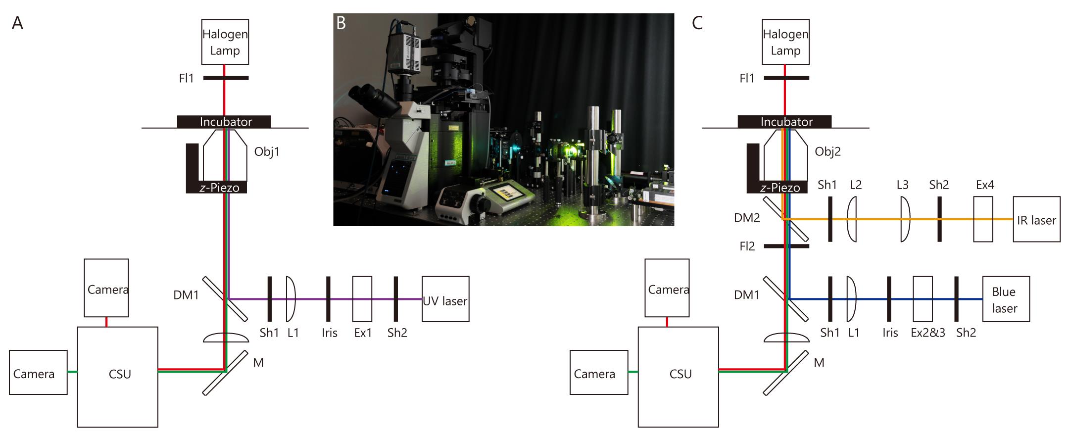
       Figure 1. Microscope and optical pathway. (A) Microscope for measurement of flow-dependent changes in ciliary shape. (B) Image of the microscope shown in A and C. Optical pathways are constructed on the optical table. (C) Microscope for optical tweezers and whole-cell fluorescence recovery after photobleaching (FRAP). For abbreviations, see Equipment section in the main text.

       
       

2. Microscope for optical tweezers and whole-cell fluorescence recovery after photobleaching (FRAP) (Figure 1B and 1C)

   1. IX83 microscope (OLYMPUS; equipped with shutter (Sh1))

   2. Spinning disk confocal unit (CSU) (Yokogawa, CSU-W1)

   3. Objective lens (Obj2): UPLSAPO 60XW 1.2 N.A. (Olympus)

   4. z-Piezo (Physik Instrumente, P-721)

   5. Digital analog converter for regulating z-Piezo (USB-DAQ) (National Instruments, USB-6363)

   6. Infrared (IR) laser for optical tweezers, 1,064 nm; 5 W (IPG Photonics, YLR-5-1064-LP-SF)

   7. Blue laser for irradiation, 488 nm; 55 mW (Coherent, Sapphire)

   8. FL1: red-right band-pass filter (Asahi, LV0630)

   9. FL2 (Asahi, SIX870)

   10. DM1 (Chroma, zt405/488/561rpc)

   11. DM2 (Chroma Technology, ZT1064rdc-sp-UF3). Note that we used ZT1064rdc-sp in Katoh et al. (2023), but that DM is better than this.

   12. Beam expander for irradiation (Ex2 and 3) (Sigmakoki, LBED-5 and LBED-3)

   13. Beam expander for optical tweezers (Ex4) (Sigmakoki, LBED-4Y)

   14. Iris (Linos G061653000) (Opened)

   15. Shutter (Sh2) (SURUGA SEIKI, model: F116)

   16. Lens for irradiation (L1) (Thorlabs, AC254-300-A)

   17. Lens for optical tweezers (L2) (Thorlabs, AC254-200-C)

   18. Lens for optical tweezers (L2) (Thorlabs, AC254-150-C)

   19. Neutral density (ND) filter for calibration of optical tweezers (only use for calibration measurement): NENIR13B (Thorlabs; transmission at 1064 nm is 3.81%)

   20. Motorized XY stage (OptoSigma, BIOS-225T and FC-101G)

   21. Stage top incubator (Tokai Hit, STXF-IX83WX and GM3000)

   22. Optical table (Nippon Boushin Industry, AS-1809)

       
       

3. Microscope for analyzing Pkd2 distribution

   1. TCS SP8 STED 3× (Leica)

   2. HC PL APO 100×/1.40 Oil STED white (Leica)

Software

1. ImageJ, Fiji (version 1.52a, NIH)

2. Excel (Microsoft)

3. Software for deconvolution of STED microscopy image (Huygens; version 21.10; Scientific Volume Imaging)

4. Software for control of IX83 and CSU (iQ; Version 3.6.3; Andor)

5. Software for control of z-Piezo (LabView 2018; Version 18.0.1f4; National instruments)

6. Software for analyzing Pkd2 distribution (Igor; version 8.0.4.2; WaveMetrics)

Procedure

1. Measurement of flow-dependent changes in ciliary shape

   1. Mouse E7.5 embryos harboring an NDE4-hsp-5HT6-mNeonGreen-2A-tdKatushka2 (Katoh et al., 2023) transgene were isolated and roller-cultured as previously described (Behringer et al., 2014).

   2. We prepared the medium for observation (see Recipes) by supplementing FluoroBrite DMEM with 75% rat serum. The medium was incubated in a CO₂ incubator.

   3. The distal portion of each embryo, including the node, was excised and placed into a chamber, consisting of a glass slide fitted with a thick silicone rubber spacer (thickness of 400 μm) to prevent disturbance of nodal flow, and covered with a coverslip (Figure 2). Setting the node region close to the glass surface is very important; however, do not deform the shape of the node to prevent disturbance of nodal flow.

      
      

      
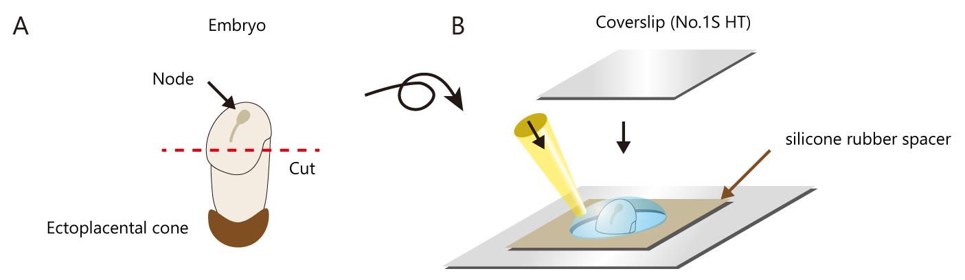
      Figure 2. Schematic of the mounting of the mouse embryonic node. (A) For imaging, the distal portion of the embryo, including the node, was carefully cut. It is preferable to cut the tissue such that the node is located at the center top of the excised tissue. For immunostaining, the ectoplacental cone was removed (see section D). (B) A silicon rubber spacer was fitted on the glass slide. Excised tissue including the node was then placed in the center of the hole with the medium. The wide bore tip is preferable for usage (see Materials and Reagents). Lastly, it was covered with a coverslip.

      
      

   4. We perform 3D live imaging using the microscope described above (see Table 1).

      Setting of the objective: The correction ring was set at 0.17 μm for 37 °C. A lens heater (37 °C) was used. Note that the deconvolution calculation (see Data analysis) is sensitive to aberrations.

      Setting z-Piezo: the z-stack distance was set to 200 nm. Typically, 301 z-stacks (60 μm) were used.

      Setting of the EM-CCD camera: EMGain and A/D were 999 and 10 MHz, respectively.

      Note: When using a high level of EM gain, do not irradiate strong light to the EM-CCD camera to prevent damage to the image sensor.

      
      

      Table 1. Equipment settings for 3D live imaging

      Device	Setting	Parameter
      Objective lens	Correction ring	0.17 μm (37 °C)
      z-Piezo	z-stack distance	200 nm
      	Range	301 z-stacks (60 μm)
      EM-CCD camera	EM gain	999
      	A/D	10 MHz

      
      

   5. The center of the node was irradiated with UV to stop the nodal flow (see Figure 1 in Katoh et al., 2023): a 375 nm laser (set at 70 mW; laser power before the objective was 23 mW) was radiated for 45 s. The irradiation duration was controlled by a shutter equipped with an IX83 microscope using iQ software. Laser protection goggles must be worn during this operation.

   6. The procedure for 3D live imaging was repeated. The settings were identical to those of the previous imaging. In most embryos, the fluorescence intensity is weak; thus, the laser power for CSU is typically higher than before UV irradiation.

      The obtained 3D images were used for analysis for flow dependent change in angle of cilia and computational mesh generation for calculating membrane tension of cilia, as described below.

   7. Measurement of PSF for deconvolution calculation (see Table 2).

      Sample: fluorescent beads were diluted 1:1,250,000 in phosphate-buffered saline [PBS(-)] solution. The beads were attached to the glass surface within several minutes.

      3D imaging of a fluorescent bead was performed using the same settings as described in step 4, excluding the use of the EM-CCD camera. To increase S/N, the EM gain and A/D of the EM-CCD camera were set to 3 and 1 MHz, respectively.

      
      

      Table 2. Equipment settings for PSF measurement

      Device	Setting	Parameter
      Objective lens	Correction ring	0.17 μm (37 °C)
      z-Piezo	z-stack distance	200 nm
      	Range	301 z-stacks (60 μm)
      EM-CCD camera	EM gain	3
      	A/D	1 MHz

      
      

2. Manipulation of single cilium by optical tweezers

   1. Mouse E7.5 embryos harboring NDE4-hsp-dsVenus-Dand5-3′-UTR (Minegishi et al., 2021) and NDE4-hsp-5HT₆-GCaMP6-2A-5HT₆-mCherry (Mizuno et al., 2020) were isolated and roller-cultured as previously described (Behringer et al., 2014).

   2. The medium was prepared as described above.

   3. The beads were prepared for trapping. Twenty microliters of polystyrene beads (diameter, 3.5 μm) were added to 980 μL of FluoroBrite DMEM (1:50 dilution). After centrifugation at 20,300× g for 15 min, isolated beads (pellets) were resuspended in 200 μL of FluoroBrite DMEM.

   4. A distal portion of each embryo, including the node, was excised and placed into a chamber consisting of a glass slide fitted with a thick silicone rubber spacer (thickness of 400 μm) to prevent any disturbance of nodal flow (see Figure 2). The embryo was carefully trimmed to obtain a node located parallel to the glass surface to prevent deformation of the embryo during observation.

      A portion of the diluted beads was carefully transferred to the medium above the node with a P2 pipette tip to expose the node to ~1–10 beads, and then carefully covered with a coverslip.

   5. Live imaging was performed, and the target cilium was set using the ciliary GCaMP6/mCherry signal. A brightfield image was observed through a red channel of the CSU to check the shape of the embryo.

   6. In the case of analysis by whole-cell FRAP later, 3D images of ciliary mCherry and cytoplasmic dsVenus were recorded (typically a z-axis depth of 1 μm with 30 sections).

   7. Mechanical stimuli were applied to cilia using the microscope described above. A polystyrene bead was trapped, placed in contact with a cilium, and forced to oscillate along the dorsoventral (D-V) axis for 1.5 h with the use of optical tweezers. Laser protection goggles must be worn during this operation.

      Setting of the objective: the correction ring was set at 0.17 μm for 37 °C. A lens heater (37 °C) was used. Please note that optical tweezers are sensitive to aberrations.

      The setting of the IR laser was 400 mW for ZT1064rdc-sp-UF3 and 800 mW for ZT1064rdc-sp (condition in Katoh et al., 2023).

      Setting z-Piezo and USB-DAQ: a 2 Hz triangle wave with 1.025 ± 0.175 V amplitude was generated using USB-DAQ controlled by the simulate signal express function in LabView and applied to the z-Piezo (Figure 3).

      Note that we manually tracked the cilium using a motorized XY stage because most embryos were displaced or deformed during 1.5 h of stimulation.

   8. To measure mRNA degradation triggered by mechanical stimuli, we performed whole-cell fluorescence recovery after photobleaching (FRAP) analysis, as described below.

   9. Measurement of trapping stiffness:

      Sample: polystyrene beads (diameter 3.5 μm) were diluted with distilled deionized water (MQ, typically 1:1,000) and placed into a flow chamber (Katoh et al., 2021) made up of a slide glass (24 mm × 60 mm, No. 1S), a coverslip (24 mm × 24 mm, No. 1S HT), and two pieces of double-sided tape for spacers (cut approximately 5 mm wide and 40 mm in length).

      Measurement: a single bead was weakly trapped by optical tweezers (typically 3.81 mW: laser power set at 100 mW and a 3.81% ND filter inserted into the optical pathway), and the restricted Brownian motion was measured. Motion of the bead was observed using a brightfield image with a CSU (using the bypath mode). Here, the frame rate needs to be faster than the cut-off frequency of the motion (we typically set this to ~200 fps).

      
      

      
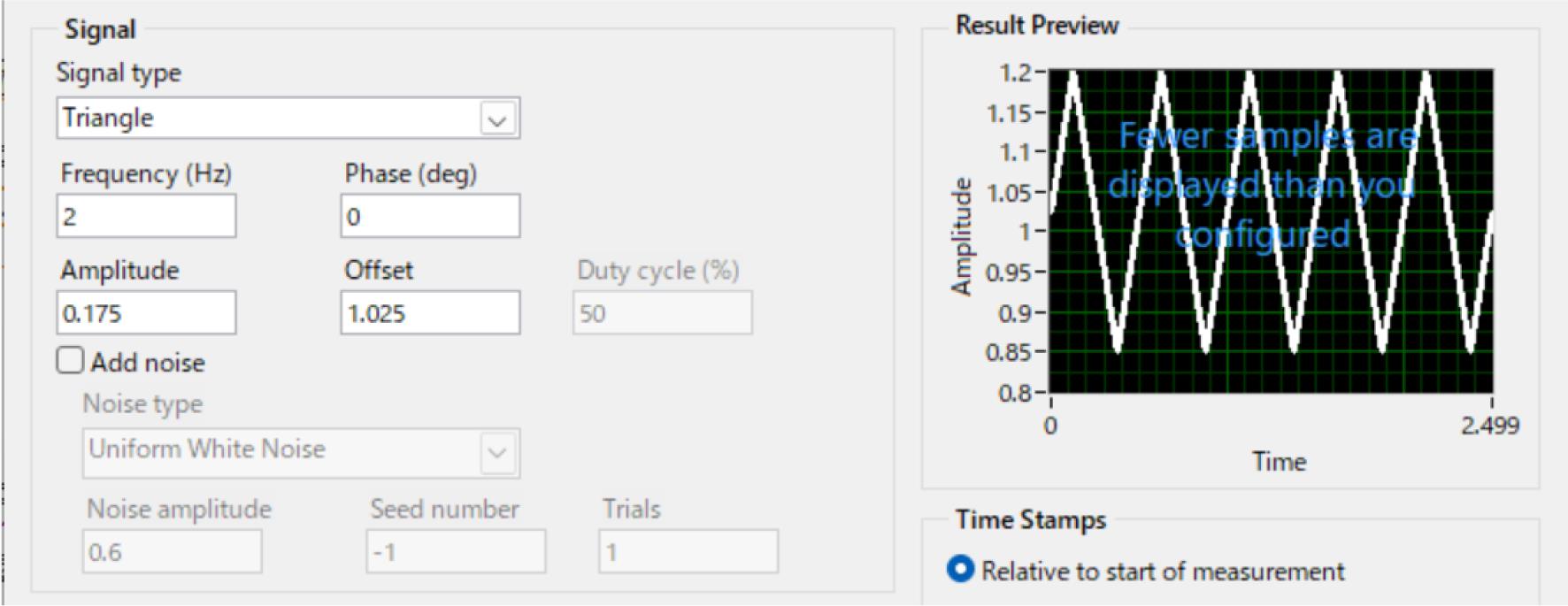
      Figure 3. Setting of simulate signal express function in LabView. z-Piezo applied a 2 Hz triangle wave with an amplitude of 1.025 ± 0.175 V using USB-DAQ.

      
      

3. Measurement of Dand5 mRNA degradation by whole-cell FRAP

   1. Whole-cell FRAP is a method for measuring mRNA levels using the level of fluorescence recovery after whole-cell bleaching (Katoh et al., 2023). Before bleaching, 3D images of ciliary mCherry and cytoplasmic dsVenus were recorded (typically, a z-axis depth of 1 μm and 30 sections; Table 3).

      
      

      Table 3. Setting of 3D live imaging for whole-cell FRAP

      Device	Setting	Parameter
      z-Piezo	z-stack distance	1 μm
      	Range	30 z-stacks (29 μm; typically)
      EM-CCD camera	EM gain	999 (typically)
      	A/D	30 MHz (typically)
      	Exposure time	200 ms (typically)
      	Binning	1 × 1

      
      

   2. All cells in the node region were uniformly bleached by 3 min irradiation with a 488 nm laser (output power set at 55 mW). The irradiation duration was controlled by a shutter equipped with an IX83 microscope using iQ software (Figure 4A). Laser protection goggles must be worn during this operation.

   3. Fluorescence recovery was measured by 3D images using the microscope described above (Figure 4B).

      Setting z-Piezo: the distance of the z-stack was set to 1 μm. Typically, 30 z-stacks (29 μm) were observed.

      Setting of the camera: the fluorescence intensity was quite low compared with that before bleaching. Therefore, we usually employed a 2 × 2 binning mode with a 1 s exposure.

      3D images were captured 15 times at 2 min time intervals (total observation duration is 30 min).

   4. Bleaching was repeated and fluorescence recovery was observed during the repeated process for 30 min (Figure 4A).

      The intensity in the second fluorescence recovery is low; thus, finally, we observed the 3D image with strong excitation (typically 30–55 mW) and long exposure times (1–4 s in each z-stack).

   5. Analysis of fluorescence recovery is described below (see “Analysis of Dand5 mRNA levels for whole-cell FRAP experiments”).

      
      

      
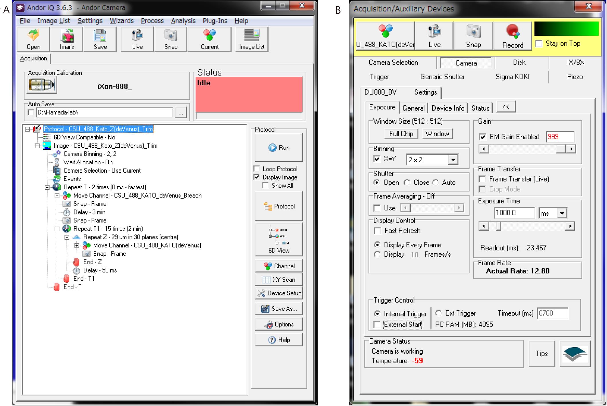
      Figure 4. Setting of iQ. (A) Screenshot of Protocol in iQ. Steps 2–4 are automatically performed using this protocol. (B) Screenshot of Channel in iQ, representing the acquisition setting in Step 3.

      
      

4. Measurement of Pkd2 distribution by 3D-STED imaging

   1. Immunostaining was performed as follows:

      1. Dissection: mouse E7.5 embryos harboring NDE2-hsp-Pkd2-Venus (Yoshiba et al., 2012) were recovered in cold PBS(-). The ectoplacental cone was then removed from the embryo (see Figure 2A). For this procedure, we recommend using a 1.5 mL tube (although other sizes work equally well).

      2. Fixation: embryos were immediately transferred to ice-cold PBS(-). When all embryos had been isolated, they were immediately fixed for 1 h at 4 °C in PBS containing 4% paraformaldehyde.

      3. Rinse: embryos were washed three times with PBS containing 0.01% Triton X-100 (PBST; see Recipes).

      4. Permeabilization: 30 min at room temperature in PBS containing 0.2% Triton X-100.

      5. Rinse: embryos were washed three times with PBST.

      6. Primary antibody: incubated overnight at 4 °C with acetylated tubulin (1:200 dilution) and green fluorescent protein (1:200 dilution) antibodies diluted in PBST.

      7. Rinse and wash: antibodies were washed three times with PBST. During this, it is preferable to change the tube. Then, wash > 6 times with PBST at 1 h intervals.

      8. Secondary antibody was incubated overnight at 4 °C with STAR RED (1:200 dilution, anti-mouse) and STAR ORANGE (1:200 dilution, anti-chick) antibodies diluted in PBST.

   2. Mounting was performed as follows:

      Mounting solution: TDE-DABCO (see Recipes)

      1. A distal portion of each embryo, including the node, was excised and the node region was placed in PBST containing 10% TDE-DABCO. In the final step, the node should be located close to the glass surface, as described below, to prevent resolution reduction—so, carefully trim the embryo.

      2. The node region was transferred to PBST containing 20% TDE-DABCO.

      3. The node region was transferred to PBST containing 50% TDE-DABCO.

      4. The node region was transferred to TDE-DABCO.

      5. The node region was placed into a chamber consisting of a glass slide fitted with a thin silicone rubber spacer (thickness 100 μm) and then carefully covered with a coverslip (see Figure 2). In this step, it is very important for the node to be close to the coverslip without deforming the shape of the node. Please note that we index-matched samples to minimize spherical aberration.

      6. Finally, it was sealed with nail polish. Samples were stored at 4 °C for approximately one week.

   3. 3D-STED observation: 3D-STED imaging was performed as follows:

      Bit depth: 16 bit

      Channel 1: excitation wavelength 561 nm (white light laser pulse), detection wavelength for HyD 571–623 nm, gating 0.3–6 ns, depletion wavelength 775 nm (pulse)

      Channel 2: excitation wavelength 633 nm (white light laser pulse), detection wavelength for HyD 650–700 nm, gating 0.3–6 ns, depletion wavelength 775 nm (pulse)

      z-donut: 60%–80% (typically 80%)

      Pinhole setting: 0.5 AU at 640 nm

      Before observation, it is better to perform Beam alignment.

      Note that in STED microscopy, the excitation light is overlapped with the STED beam, quenching excited molecules in the excitation spot periphery. In this setting, we used the same wavelength of the STED beam for Channel 1 and Channel 2 (see depletion wavelength), so chromatic aberration does not occur.

   4. Analysis of 3D images is described below in Analysis of Pkd2 distribution for STED images.

Data analysis

1. Analysis for flow dependent change in angle of cilia

   1. Deconvolution calculation of 3D images: 3D deconvolution calculations were performed using DeconvolutionLab2 (Sage et al., 2017) (Figure 5A).

      Settings of DeconvolutionLab2:

      Algorithm: Richardson-Lucy Total Variation

      Iterations (N): 100

      Regularization parameter λ: 10^-12

      
      

      
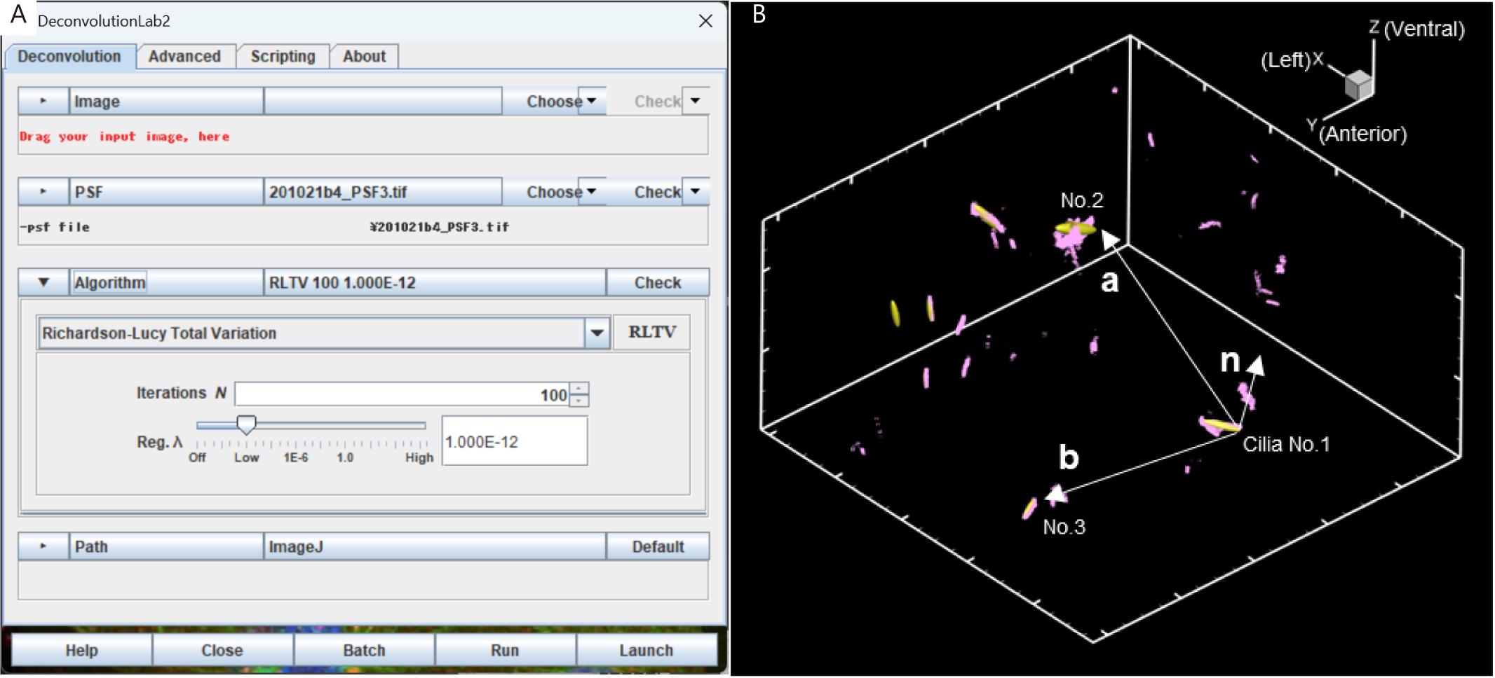
      Figure 5. Setting for deconvolution and correction of the three-dimensional orientation of the embryo. (A) Screenshot of DeconvolutionLab2. (B) Define two vectors a and b from the base positions of the three cilia and calculate their outer product n = a × b. The same process is applied to two different images (before and after UV irradiation) and the images are corrected so that the respective n-vectors match.

      
      

   2. An 8-bit transformation of the image was performed and location information on the ciliated surface was extracted from ImageJ’s Gaussian Filter and Find Edges convolution functions.

   3. To quantify the three-dimensional orientation of the embryo, the basal positions of the three cilia were detected, which were defined as r₁, r₂, and r₃.

   4. Two vectors, a (= r₂ - r₁) and b (= r₃ - r₁), were defined from the three basal positions, as shown in Figure 5B, and one normal vector, n = a × b, was determined by the outer product of these vectors.

   5. The n-vector in both the pre- and post-UV irradiation images was found, and these images were then rotated such that the two n-vectors coincide.

   6. Ellipsoid fitting was performed on the ciliary geometry obtained from the microscopic images. The ciliary posture was defined by determining the declination of the ellipsoid major axis with respect to the dorsoventral axis.

   7. Ciliary deformation was defined based on the change in the angle before and after UV irradiation.

      
      

2. Computational mesh generation for calculating membrane tension of cilia

   1. The cross-sectional centers of the cilia in the z-stack of each 3D image were determined.

   2. Spline interpolation was applied to represent a smooth curve connecting the centers of each z-section.

   3. We defined circles of radius 100 nm each in the direction normal to the centerline, as shown in Figure 6.

      
      

      
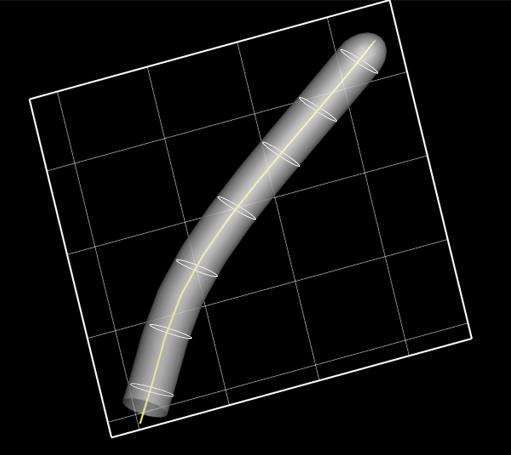
      Figure 6. Computational mesh generation to represent the ciliated membrane surface. The ciliated surface is represented as a cylindrical surface with a series of circles of radius 100 nm normal to the centerline (yellow line). Grid size, 1.6 µm.

      
      

   4. The surface of the ciliary membrane was defined by connecting each circumference in the direction of the longitudinal axis.

   5. A computational mesh was generated by discretizing the defined membrane surface by triangles.

   6. The cilia shape after UV irradiation was defined as the reference shape and the shape before UV irradiation was used to calculate the elastic deformation of the cilia.

      
      

3. Analysis of Dand5 mRNA levels for whole-cell FRAP experiments

   1. As described in Figure S6 and the Methods section in Katoh et al. (2023), our whole-cell FRAP system with NDE4-hsp-dsVenus-Dand5-3′-UTR transgene (Minegishi et al., 2021) can directly measure Dand5 mRNA levels as the final (plateau) intensity. In this analysis, we used three 3D images: the image captured before stimuli, the last image of first fluorescence recovery, and the final image of second fluorescence recovery.

   2. Measurement of intensity before stimulation:

      1. We first find a cell with a stimulated cilium and neighboring unstimulated ciliated cells (typically two unstimulated cells).

      2. The suitable size of the region of interest (ROI) for these cells was set, and the average intensity in each of them was measured using ImageJ/Fiji.

      3. The background intensity was measured using the region in the center of the node.

      4. Finally, we calculated the following ratio: Ratio₀ = 2 (I_S - I_B)/(I_N1 + I_N2 - 2I_B), where I_S, I_B, I_N1, and I_N2 are the intensity in stimulated cells, background intensity, intensity in neighboring unstimulated cell number #1, and intensity in neighboring unstimulated cell number #2, respectively.

   3. Measurement of the intensity in the last image of first fluorescence recovery.

      1. The stimulated cilium and the unstimulated cells were carefully identified. This was difficult because embryos are usually deformed during long-term observations. To identify target cells, we used movies taken during optical tweezer experiments, and 3D timelapse images during the FRAP experiment.

      2. The intensity of each cell and the background intensity were measured as described above. We then calculated the Ratio₁ as described above.

   4. Measurement of the intensity in the final image of second fluorescence recovery:

      The cells were carefully identified, the intensity of each cell was measured, and the background intensity was measured as described above. We then calculated Ratio₂, as described above.

   5. Finally, the normalized values were calculated: mRNA levels 30 min after stimuli (%) = Ratio₁/Ratio₀, mRNA levels 1 h after stimuli (%) = Ratio₂/Ratio₀

      
      

4. Analysis of Pkd2 distribution for STED imaging

   1. Deconvolution calculation by Huygens software

      1. Firstly, we directly read a .lif file by Huygens and then started the deconvolution wizard.

         The settings of the deconvolution wizard were as follows:

         Stabilization: On

         Deconvolution algorithm: classical maximum likelihood estimation (CMLE)

         PSF estimation: as close guess, Max detail

      2. The calculated image was saved.

         A higher bit depth is better for subsequent analysis; therefore, we save the image as a .ome file in Huygens. The file was then opened by Fiji. When the image is opened by Fiji, it is flipped vertically, so we should reflip vertically. This image was saved as a .tiff file.

   2. Analysis of angular distribution

      We used a custom-written macro that runs in Igor software. The details of this macro are as follows:

      1. First, using ImageJ, the location of a single cilium in a 3D image was memorized as the width, depth, height, x, y, and z values of the ROI. The threshold values in the red and green channels were measured to extract the signal. Then, the 3D tiff image was loaded with Igor.

      2. When the cilium elongates along the z-axis, we calculated the center of gravity of the red channel in each xy plane (each z-stack). We typically use the threshold value for the red channel as the background. However, the background affects this calculation; therefore, it is preferable to carefully set the background. The resulting (x, y) coordinates represent the cilium center in each z-stack.

         When the cilium elongates along the x- or y-axis, we calculated the center in yz or xz planes using the same method.

      3. The angle of the Pkd2 channel was calculated. If the z-plane had a Pkd2 signal above the threshold, we calculated the following and saved it as an array.

         Angle from the center of the cilia to the Pkd2 signal using arctangent function θ

         Distance from the center of cilia to the Pkd2 signal: r

         Intensity: I

      4. The intensity was accumulated at each angle in each cilium. We extracted pixels whose r was close to the cilium (we usually set 500–1,000 nm) to exclude the non-ciliary signal. Then, all I values are accumulated at each θ angle (typically a 45° sector) in every cilium.

      5. All data from each cilium were plotted in one figure such as Figure 4B in Katoh et al. (2023).

Recipes

1. Medium for observation: FluoroBrite DMEM supplemented with 75% rat serum

   We usually store 1 mL of 100% rat serum in sterile tubes at -80 °C and 10 mL of FluoroBrite DMEM in Corning tubes at 4 °C (long-term storage at -80 °C). Just before use, we mix 3 mL of rat serum with 1 mL of FluoroBrite DMEM on a clean bench.

   
   

2. PBST

   100 μL of Triton X-100

   1 L of PBS(-)

   
   

3. TDE-DABCO

   11.5 g of TDE

   250 μL of DABCO

   150 μL of 1 M Tris-HCl (pH 8.0)

Acknowledgments

We thank K. Mizuno, K. Minegish, X. Sai, and all members of the Laboratory for Organismal Patterning for improving the protocol; K. Kawaguchi and members of his laboratory for support in developing the analysis method for Pkd2 distribution for STED images; and D. Takao for support with STED imaging.

This study was supported by grants from the Ministry of Education, Culture, Sports, Science, and Technology (MEXT) of Japan (No. 17H01435) and Core Research for Evolutional Science and Technology (CREST) of the Japan Science and Technology Agency (JST) (No. JPMJCR13W5) to H.H.; by a Grant-in-Aid (No. 21K15096) from the Japan Society for the Promotion of Science (JSPS); by the RIKEN Special Postdoctoral Researcher Program to T.A.K.; by a grant from Precursory Research for Embryonic Science and Technology (PRESTO) of JST (No. JPMJPR2142) to T.O. 3D-STED microscopy was supported by grants from JST (Nos. JPMJMS2025-14, JPMJCR20E2, JPMJCR15G2, and JPMJCR1852), and JSPS (Nos. 19H05794 and 16H06280) to Y.O.

This protocol is derived from the original research paper (Katoh et al., 2023).

Competing interests

The authors declare no competing interests.

Ethical considerations

All animal experiments were approved by the Institutional Animal Care and Use Committee of RIKEN Kobe Branch.

References

1. Ashkin, A. (1970). Acceleration and Trapping of Particles by Radiation Pressure. Phys Rev Lett 24(4): 156-159.
2. Behringer, R., Gertsenstein, M., Nagy, K. V. and Nagy, A. (2014). Manipulating the mouse embryo: a laboratory manual. Cold Spring Harbor Laboratory Press. ISBN: 9781936113002, 9781936113019.
3. Ferreira, R. R., Fukui, H., Chow, R., Vilfan, A. and Vermot, J. (2019). The cilium as a force sensor-myth versus reality. J Cell Sci 132(14): jcs213496.
4. Katoh, T. A., Daiho, T., Yamasaki, K., Danko, S., Fujimura, S. and Suzuki, H. (2021). Angle change of the A-domain in a single SERCA1a molecule detected by defocused orientation imaging. Sci Rep 11(1): 13672.
5. Katoh, T. A., Ikegami, K., Uchida, N., Iwase, T., Nakane, D., Masaike, T., Setou, M. and Nishizaka, T. (2018). Three-dimensional tracking of microbeads attached to the tip of single isolated tracheal cilia beating under external load. Sci Rep 8(1): 15562.
6. Katoh, T. A., Omori, T., Mizuno, K., Sai, X., Minegishi, K., Ikawa, Y., Nishimura, H., Itabashi, T., Kajikawa, E., Hiver, S., et al. (2023). Immotile cilia mechanically sense the direction of fluid flow for left-right determination. Science 379(6627): 66-71.
7. Klar, T. A., Jakobs, S., Dyba, M., Egner, A. and Hell, S. W. (2000). Fluorescence microscopy with diffraction resolution barrier broken by stimulated emission. Proc Natl Acad Sci U S A 97(15): 8206-8210.
8. Minegishi, K., Rothe, B., Komatsu, K. R., Ono, H., Ikawa, Y., Nishimura, H., Katoh, T. A., Kajikawa, E., Sai, X., Miyashita, E., et al. (2021). Fluid flow-induced left-right asymmetric decay of Dand5 mRNA in the mouse embryo requires a Bicc1-Ccr4 RNA degradation complex. Nat Commun 12(1): 4071.
9. Mizuno, K., Shiozawa, K., Katoh, T. A., Minegishi, K., Ide, T., Ikawa, Y., Nishimura, H., Takaoka, K., Itabashi, T., Iwane, A. H., et al. (2020). Role of Ca²⁺ transients at the node of the mouse embryo in breaking of left-right symmetry. Sci Adv 6(30): eaba1195.
10. Nauli, S. M., Alenghat, F. J., Luo, Y., Williams, E., Vassilev, P., Li, X., Elia, A. E., Lu, W., Brown, E. M., Quinn, S. J., et al. (2003). Polycystins 1 and 2 mediate mechanosensation in the primary cilium of kidney cells. Nat Genet 33(2): 129-137.
11. Omori, T., Winter, K., Shinohara, K., Hamada, H. and Ishikawa, T. (2018). Simulation of the nodal flow of mutant embryos with a small number of cilia: comparison of mechanosensing and vesicle transport hypotheses. R Soc Open Sci 5(8): 180601.
12. Praetorius, H. A. and Spring, K. R. (2001). Bending the MDCK Cell Primary Cilium Increases Intracellular Calcium. J Membr Biol 184(1): 71-79.
13. Rydholm, S., Zwartz, G., Kowalewski, J. M., Kamali-Zare, P., Frisk, T. and Brismar, H. (2010). Mechanical properties of primary cilia regulate the response to fluid flow. Am J Physiol Renal Physiol 298(5): F1096-1102.
14. Sage, D., Donati, L., Soulez, F., Fortun, D., Schmit, G., Seitz, A., Guiet, R., Vonesch, C. and Unser, M. (2017). DeconvolutionLab2: An open-source software for deconvolution microscopy. Methods 115: 28-41.
15. Shinohara, K. and Hamada, H. (2017). Cilia in Left-Right Symmetry Breaking. Cold Spring Harb Perspect Biol 9(10): a028282.
16. Su, S., Phua, S. C., DeRose, R., Chiba, S., Narita, K., Kalugin, P. N., Katada, T., Kontani, K., Takeda, S. and Inoue, T. (2013). Genetically encoded calcium indicator illuminates calcium dynamics in primary cilia. Nat Methods 10(11): 1105-1107.
17. Vicidomini, G., Moneron, G., Han, K. Y., Westphal, V., Ta, H., Reuss, M., Engelhardt, J., Eggeling, C. and Hell, S. W. (2011). Sharper low-power STED nanoscopy by time gating. Nat Methods 8(7): 571-573.
18. Yoshiba, S., Shiratori, H., Kuo, I. Y., Kawasumi, A., Shinohara, K., Nonaka, S., Asai, Y., Sasaki, G., Belo, J. A., Sasaki, H., et al. (2012). Cilia at the node of mouse embryos sense fluid flow for left-right determination via Pkd2.Science 338(6104): 226-231.