- Protocols

- Articles and Issues
- For Authors
- About
- Become a Reviewer

Imaging Membrane Proteins Using Total Internal Reflection Fluorescence Microscopy (TIRFM) in Mammalian Cells
Published: Vol 13, Iss 4, Feb 20, 2023 DOI: 10.21769/BioProtoc.4614 Views: 2016
Reviewed by: Chiara AmbrogioSoumya MoonjelyAnonymous reviewer(s)
Original research article
The authors used this protocol in:

May 2022
Advertisement


Protocol Collections
Comprehensive collections of detailed, peer-reviewed protocols focusing on specific topics


Related protocols
Abstract
The cell surfaceome is of vital importance across physiology, developmental biology, and disease states alike. The precise identification of proteins and their regulatory mechanisms at the cell membrane has been challenging and is typically determined using confocal microscopy, two-photon microscopy, or total internal reflection fluorescence microscopy (TIRFM). Of these, TIRFM is the most precise, as it harnesses the generation of a spatially delimited evanescent wave at the interface of two surfaces with distinct refractive indices. The limited penetration of the evanescent wave illuminates a narrow specimen field, which facilitates the localization of fluorescently tagged proteins at the cell membrane but not inside of the cell. In addition to constraining the depth of the image, TIRFM also significantly enhances the signal-to-noise ratio, which is particularly valuable in the study of live cells. Here, we detail a protocol for micromirror TIRFM analysis of optogenetically activated protein kinase C-ϵ in HEK293-T cells, as well as data analysis to demonstrate the translocation of this construct to the cell-surface following optogenetic activation.
Graphic abstract
Background
Total internal reflection (TIR) occurs when the angle of incidence of a beam of light upon a refractive surface exceeds a certain threshold, called the critical angle, resulting in reflection of the incident beam of light. While this implies an absence of transmission of light across the interface, there is an escape of electromagnetic energy in the form of an evanescent wave. Total internal reflection fluorescence microscopy (TIRFM) relies on this exponentially decaying evanescent wave that penetrates to a depth of ~100 nm into the sample area. Given that TIR occurs at the interface of two materials with distinct refractive indices, in cell biology experiments the result is that the evanescent wave will only excite fluorescence capable moieties in the evanescent field at or near the cell surface. Thus, TIRFM illuminates fluorescent particles at the cell membrane below the Rayleigh limit for resolution, making the technique well suited for the study of membrane proteins and membrane-delimited signaling events, in fixed or live cell samples.
Several types of microscopy are utilized in the literature to achieve optical sectioning with the intent to localize fluorescent biological moieties to various cellular fractions. Confocal microscopy is a common and versatile technique that has the potential to target any plane of the sample rather than only the glass/liquid interface, as in TIRFM. As with any microscopy, the resolution is determined by the lateral (X-Y) and axial dimensions of the imaging voxel (the Z-plane of a 3-dimensional pixel), each of which is dependent upon numerous factors. Thus, the resolution of the image is determined by the hardware (lens and detector), software, and sample preparation, as well as the fluorophore (protein or dye) and the light source in use. Commonplace confocal microscopes typically operate with a lateral dimension above the Abbe limit of ~250 nm. However, adaptations such as Airy disc scanners and stimulated emission dyes that form the basis of many super resolution techniques can reduce the lateral dimension to below 100 nm. Technologies such as Airy disc confocal, stimulated emission depletion, photoactivated localization microscopy, and stochastic optical reconstruction microscopy have yielded unprecedented information about subcellular architecture and protein localization (Vangindertael et al., 2018). However, they typically require a fixed sample (particularly where specific emission dyes must be employed) and have lower axial resolution (equivalent to the depth of the slice of up to ~500 nm) (Axelrod, 2001) and imaging speeds that are below the biological timescale. The issue of low axial resolution can be improved with two-photon localization microscopy, which, in some cases, can be combined with super resolution in the X-Y plane (Zong et al., 2017). However, this suite of tools is typically expensive and requires specialized hardware, software, and sample preparation. In contrast, TIRFM provides precise localization of fluorescence moieties, at or close to the cell membrane (axial resolution below ~100 nm). In addition to being commercially available, TIRFM systems can be homemade and constructed to image a range of user-preferred fluorophores, including genetically encoded fluorescent proteins, in live cells at relatively high speed in a cost-effective manner. Therefore, TIRFM is the imaging modality of choice to study membrane-delimited proteins with a high signal-to-noise ratio in fixed and live samples.
Materials and Reagents
Lens cleaning tissue (Thor Labs, catalog number: MC-50E)
#1.5 coverslip (Warner Instruments, catalog number: CS-15R)
35 mm tissue culture-treated dishes (Fisherbrand, Fisher Scientific, catalog number: FB012920)
60 mm tissue culture-treated dishes (Fisherbrand, Fisher Scientific, catalog number: FB012921)
Immersion oil (Cargille Laboratories, catalog number: 16241)
Dulbecco’s modified Eagle medium (ATCC, catalog number: 30-2002)
OptiMEM (Gibco, catalog number: 02634)
0.05% trypsin (Cytiva, catalog number: SH30236.01)
Polyethylenimine (PEI) (Polysciences, catalog number: 24765-1)
Human embryonic kidney 293-T cells (ATCC, catalog number: CRL-3216)
Fetal bovine serum (R&D Systems, catalog number: S12450)
Penicillin/streptomycin (Cytiva, catalog number: SV30010)
CIBN-CAAX (Dr. Pietro De Camilli, Addgene ID# 79574)
mCherry-CRY2-5PtaseOCRL (Dr. Pietro De Camilli, Addgene ID# 66836)
mCherry-CRY2–mPKCϵ-CAT-HA (Gada et al., 2022, Addgene ID# 190483)
NaCl (Fisher, catalog number: S271)
KCl (Fisher, catalog number: P217)
MgCl2 (Fisher, catalog number: M33)
CaCl2 (Fisher, catalog number: C79)
HEPES (Oakwood Chemical, catalog number: 047861)
TIRF imaging solution (see Recipes)
Equipment
Lasers (Coherent, OBIS LX445 1185051, OBIS LS 561 1253301)
Camera (Teledyne Photometrics, Prime95B)
Stage (Mad City Labs, X-Y-Z nanopositioning, model: Nano-LPS)
Any in-house or commercial microscope frame that can be modified to hold micromirrors below the objective lens. We use an RM21 frame from Mad City Labs Inc.
Micromirrors are available from Mad City Labs
High numerical aperture (NA) objective lens (e.g., Olympus 60×, 1.5 NA from Olympus)
Quick release magnetic sample holder (Warner Instruments, model: QR-42LP)
Software
Micromanager (University of California at San Francisco, https://micro-manager.org)
ImageJ (National Institute of Health/Wayne Rasband, https://imagej.nih.gov/ij/). Alternatively, use FIJI (ImageJ) software; a build of ImageJ with several prepopulated Plugins and Macros for data analysis.
Procedure
In this protocol, experimental analyses of mCherry-CRY2–mPKCϵ-CAT-HA, CIBN-CAAX, and mCherry-CRY2-5PtaseOCRL are used as an example. mCherry-CRY2–mPKCϵ-CAT-HA was developed and utilized in Gada et al. (2022); CIBN-CAAX and mCherry-CRY2-5PtaseOCRL were developed and demonstrated in Idevall-Hagren et al. (2012). Briefly, CRY2-CIBN are protein partners that form a light-controlled dimerization system consisting of cryptochrome 2 (CRY2) and CIBN, the N-terminal region of the transcription factor, CIB1. CIBN is anchored to the membrane with a C-terminal CAAX box (Liu et al., 2008; Idevall-Hagren et al., 2012). Following blue-light illumination, CRY2 absorbs a FAD molecule, undergoing a conformational change that promotes binding to CIBN, resulting in CRY2 and its cargo (in this case, mPKCϵ-CAT-HA) being targeted to the membrane.
Equipment setup
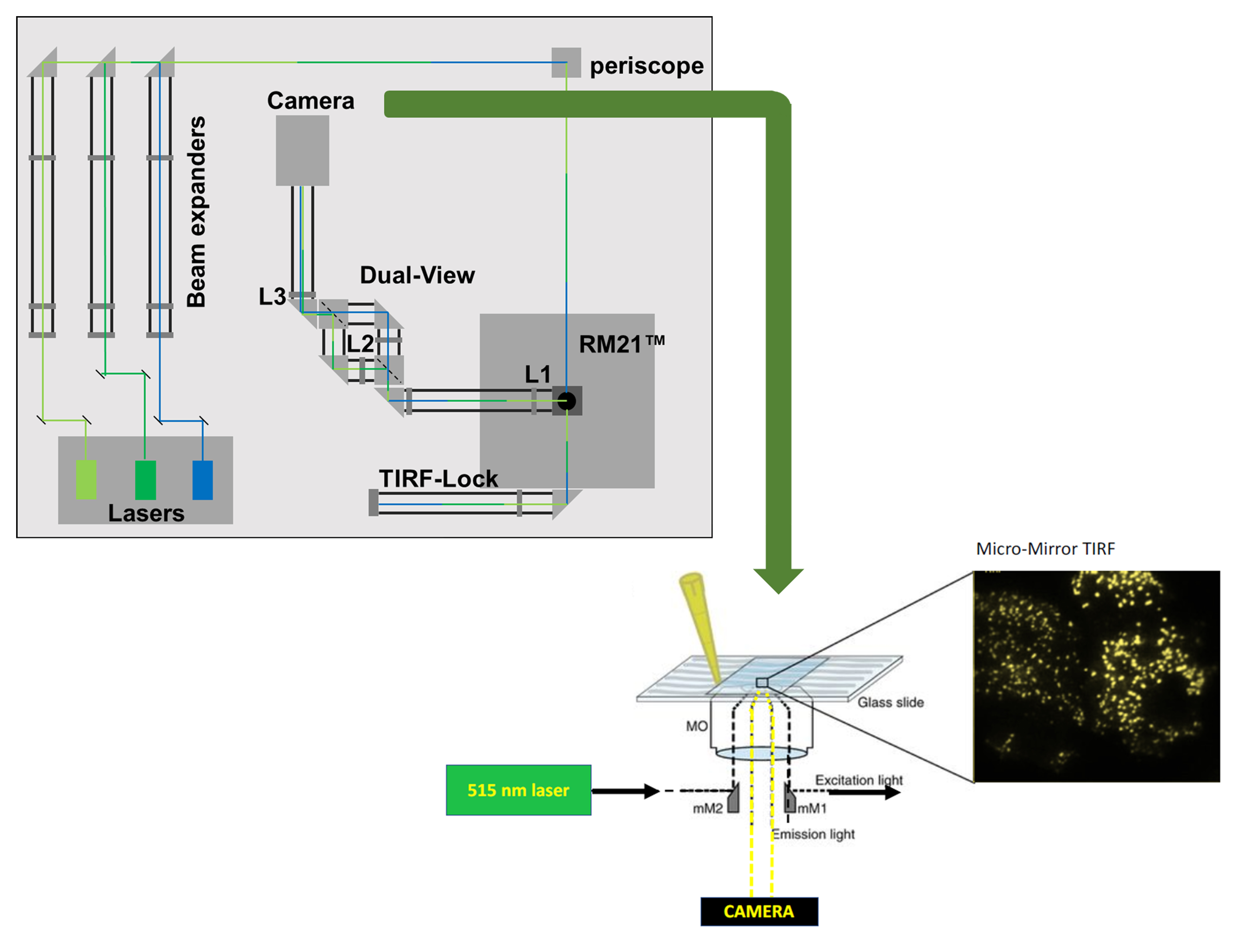
The assembly of a micromirror TIRF microscope was described by Larson et al. (2014) and this formed the basis of our equipment setup. Lasers for TIRFM are selected based on their ability to provide a continuous beam centered on the appropriate excitation wavelength(s) required for the study. We typically employ lasers that can be modulated to vary the output power according to the experimental conditions [e.g., Coherent OBIS solid-state diode lasers that operate with an output between 5–150 mW (wavelength dependent)]. Laser beams are conditioned for coherence with custom-built Keplerian beam expanders upstream of laser cleanup filters. Here, we excite monomeric Cherry (mCherry), and so employ a 561 nm cleanup filter with a bandwidth of 10 nm (561/10 nm). Laser alignment and independent verification of the output are obtained using an optical power meter that can be placed in the beam path. Multiple laser lines can be added to the system with appropriate cleanup filters. For example, we also use 445 and 514 nm lasers with 445/10 nm and 514/10nm cleanup filters, respectively, downstream of the 561 laser. Such arrangement allows for a broad range of applications with multicolor imaging. The 445 nm laser can be used to activate the optogenetic probes described in this protocol. Following expansion to ~8 mm, the laser line(s) are combined into a single coherent incident beam that is focused onto the micromirror positioned below the TIRF lens (Figure 1). We use a high numerical aperture apochromat objective [60×, 1.5 numerical aperture (NA); Olympus] mounted on an open-microscope frame equipped with a piezo-driven nanopositioning stage (Mad City Labs, Inc).
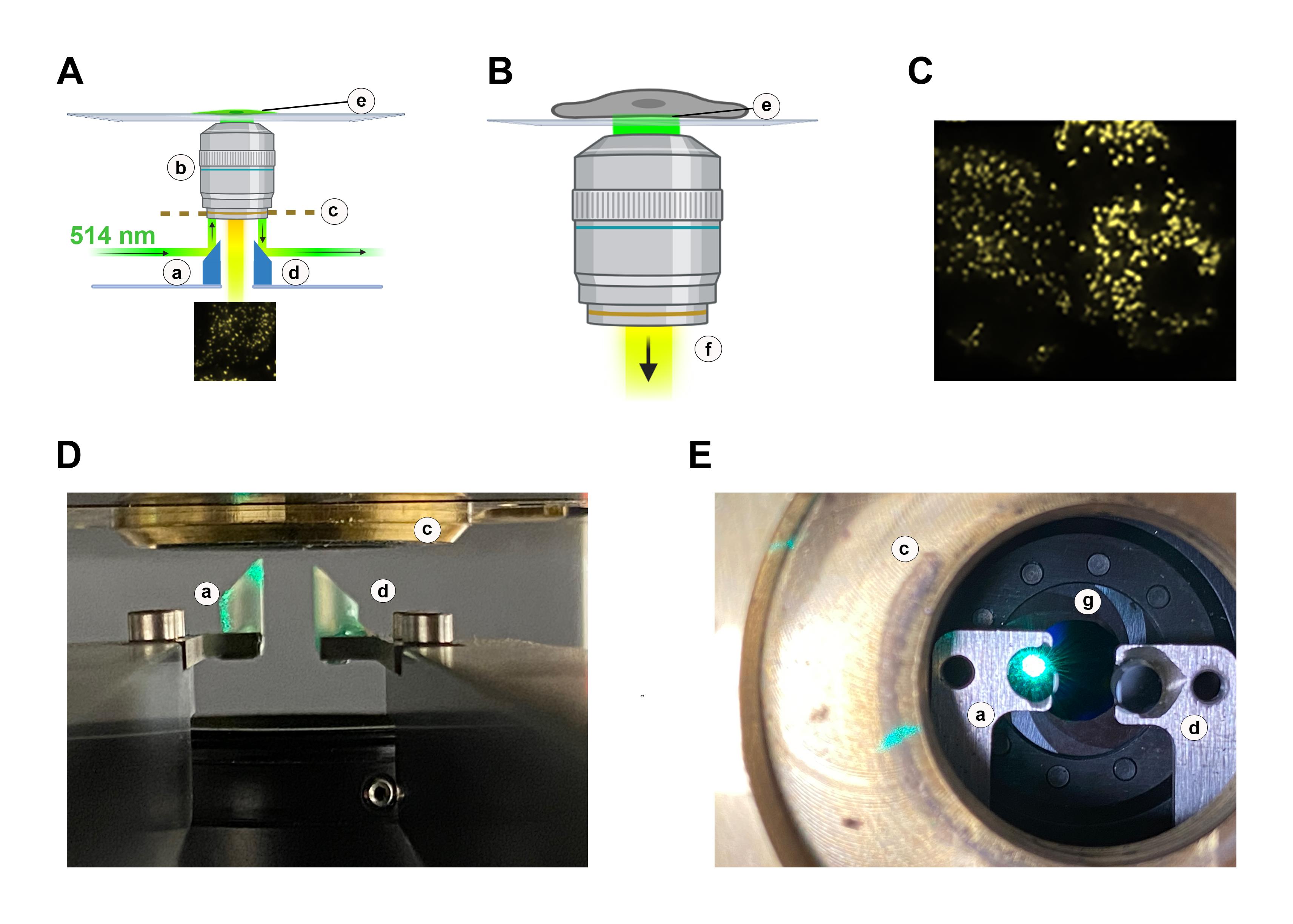
Figure 1. A schematic representation of micromirror TIRF. A. Schematic showing a 514 nm laser line entering the microscope frame horizontally, below the lens. The coherent beam is reflected 90° by a micromirror held on an arm (a), into the TIRF objective lens (b). The lens is held in a threaded mount (c), and a second micromirror (d) bounces the exit beam away from the sample area. The system is adjusted to create an evanescent wave (e) that penetrates ~100 nm from the interface between the glass coverslip and the sample. B. A closeup showing that the evanescent wave (e) does not penetrate the cytoplasm of the cell of interest. Fluorophores excited by the evanescent wave formed by the 514 nm excitation laser beam (i.e., yellow fluorescent proteins such as eYFP and mVenus) emit a yellow light that penetrates the central optical axis of the TIRF lens (f) and is ultimately collected by a detector. C. Example image showing individual YFP-tagged membrane proteins captured at the surface of a cell studied in TIRF mode using the setup described. D. Photograph of the micromirrors (a, d) positioned below the TIRF objective. The excitation beam is reflected 90° by the first micromirror (a), into the lens. The lens is held in a threaded mount (c) and is reflected 90° away from the sample area. The fluorescence signal, not visible, passes between the micromirrors along the central axis of the lens. E, Photograph of the micromirrors from above with the lens removed. The entry and exit micromirrors (a, d) are visible, with the 514 nm excitation beam shown reflecting off the entry micromirror (a). Each micromirror is mounted on an arm below the threaded mount (c) that holds the lens. Fluorescence signal from the sample will pass between the micromirrors along the central axis of the lens through a ring diaphragm that is positioned below the micromirrors (g).We use an RM21 microscope frame from Mad City Labs Inc; however, any microscope frame (including older commercial systems) that can be modified to accommodate micromirrors below the objective lens is suitable. One micromirror is placed in the beam path, directly below the leading edge of the objective lens. Micromirrors are also available from Mad City Labs Inc. Adjusting the position of the mirror beneath the lens controls the angle at which the excitation beam enters the lens and thereby the depth of the evanescent wave and the exit position of the beam from the lens (see the graphical abstract for a visualization of the setup). The relative position of the micromirror and lens is adjusted to modify how light refracts at the interface with the cells. For experiments, the lens is paired with very low autofluorescence immersion oil that has a similar refractive index [e.g., Cargille Type LDF (refractive index of 1.5)]. For our studies, the emission of mCherry is isolated from the excitation beam by an exit micromirror placed below the lens, opposite from the entry mirror (graphical abstract). A ring diaphragm positioned below the micromirror assembly further reduces crosstalk between the laser and the emission signal from the fluorophores. When the emission signal contains fluorescence from two fluorophores, the beam is separated into two parallel tracks using a beam splitter comprised of two 510 nm long pass filters. The peak emission of mCherry is above 510 nm. Downstream of this, mCherry is imaged through a 620/60 nm bandpass filter and the signal from the fluor is then captured on a back-illuminated sCMOS camera (Teledyne Photometrics). In studies using a second fluorophore that emits below 510 nm, the emission is directed to an appropriate bandpass filter on the other arm of the beam splitter. In each case, the laser output and the camera are controlled by Micro-Manager freeware (University of California San Francisco). All filters and mirrors are from Chroma. Lenses, pinholes, diaphragms, and the power meter are from Thor-Labs. TetraSpeck beads (Thermo) are routinely imaged to map the sCMOS chip and calibrate the evanescent field depth to 100 nm.
Cell seeding
Culture HEK-293 cells in 10 cm tissue culture-treated dishes in growth media containing phenol red–free Dulbecco’s modified Eagle medium (DMEM) supplemented with 1% penicillin/streptomycin and 10% fetal bovine serum and maintained at 5% CO2 at 37 °C.
After cells are ~70% confluent, remove growth media and replace with 1 mL of 0.05% trypsin for 1–2 min.
When cells have detached from the dish, place a few isolated drops (~5–8 µL total) of trypsinized cell suspension on a 15 mm #1.5 coverslip in a 35 mm dish (Figure 2).
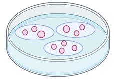
Figure 2. Cell seeding procedure for glass coverslips to obtain single cells in certain areasAfter ~1 min, add 2 mL of growth media (as in step B1) to the 35 mm dish and incubate overnight.
Cell transfection
Ensure that cells cover 30%–50% of the area of the coverslip prior to transfection.
Mix plasmid DNA of constructs for study in 50 µL of OptiMEM or any low serum, antibiotic-free media in a centrifuge tube.
In another tube, add the transfection reagent PEI in a 1:4 ratio of DNA:PEI and combine the contents of both tubes. We transfected 0.75 μg each of mCherry-CRY2–mPKCϵ-CAT-HA and CIBN–CAAX or mCherry-CRY2-5PtaseOCRL and CIBN-CAAX.
Cells for experiments that are performed to estimate background can be transfected with 0.75 μg of CIBN-CAAX only.
Incubate the transfection solution for 20 min.
Remove growth media from cells and replace with 1 mL of OptiMEM.
Add the transfection solution to the seeded cells and incubate for 2–3 h.
Remove transfection media and replace with 2 mL of growth media per 35 mm culture dish.
Incubate overnight at 37 °C and 5% CO2.
Experimental setup and data acquisition
To prepare the TIRF setup, gently wipe off the lens with lens cleaning tissue and place a drop of immersion oil on the lens.
Set the exposure time to 100 ms to best capture the fluorescence without causing photobleaching of the fluorophore.
Set the movie parameters under the data acquisition function in Micromanager to acquire data every 2–5 s for 500 frames.
Enter the data file path for the storage disc location on which the data will be stored and set the storage mode to data stacks.
Mount a coverslip on the sample stage by placing it within the holder (Figure 3), rotating the top to align the magnetic lock, and seal the coverslip into place.
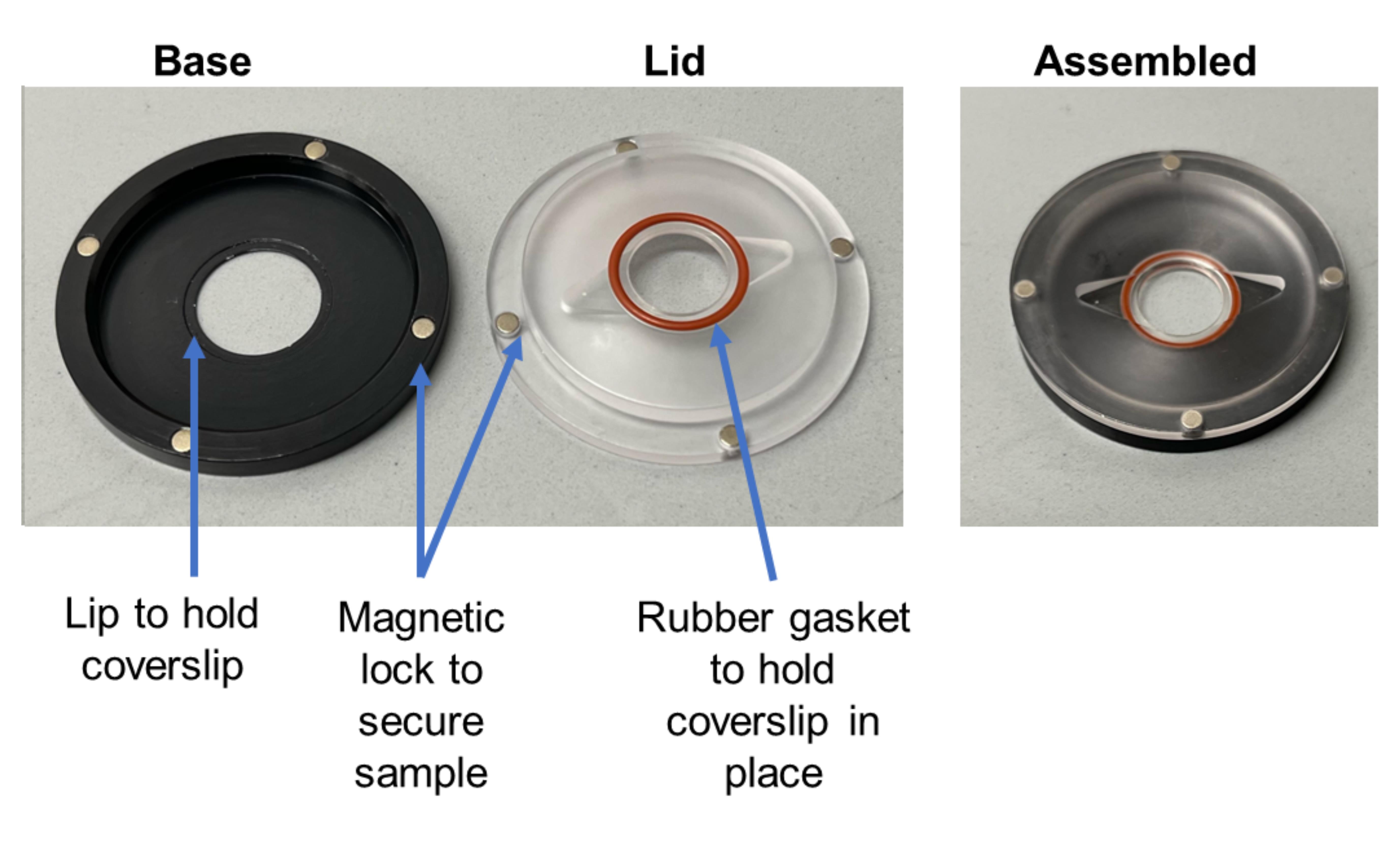
Figure 3. Sample holder assembly. A quick release magnetic sample holder for circular, 15 mm coverslips of 1.5 mm thickness from Warner Instruments (left). Assembly of sample holder (right).Gently add 150 µL of TIRF imaging solution on top of the coverslip, ensuring that cells are not sheared off the glass in the process.
Place the sample holder on the stage and adjust the stage height using Micromanager so that the cells on the coverslip are visible under white transmitted light. Cells appear close together in some regions while remaining well-spaced in some areas.
Under dim ambient light, set the 561 nm laser to a low power (~20%) to visualize the mCherry in cells that have been successfully transfected and select suitable cells for analysis.
Initiate data acquisition with the 561 nm laser set at 50% power (or less), to prevent photobleaching of the fluorophore.
After two to three frames have been captured, turn on the 445 nm laser at full power to trigger mCherry-CRY2-mPKCϵCAT-HA or mCherry-CRY2-5PtaseOCRL recruitment to the cell surface, macroscopically assessed by an increase in mCherry fluorescence at the cell surface through the course of data acquisition. A common 488 nm laser line can also be used here.
Once data acquisition is complete, save the file in TIF format, place both lasers on standby mode, and replace the coverslip to begin data acquisition from another cell.
Image cells transfected only with CIBN-CAAX for background signal using the same experimental protocol and lasers as the mCherry-tagged constructs. The mean fluorescence signal from the background is subtracted from the mCherry fluorescence measurements.
Data analysis
Launch ImageJ (or FIJI) computer program (Figure 4).
In ImageJ, open the TIF file (Figure 4).
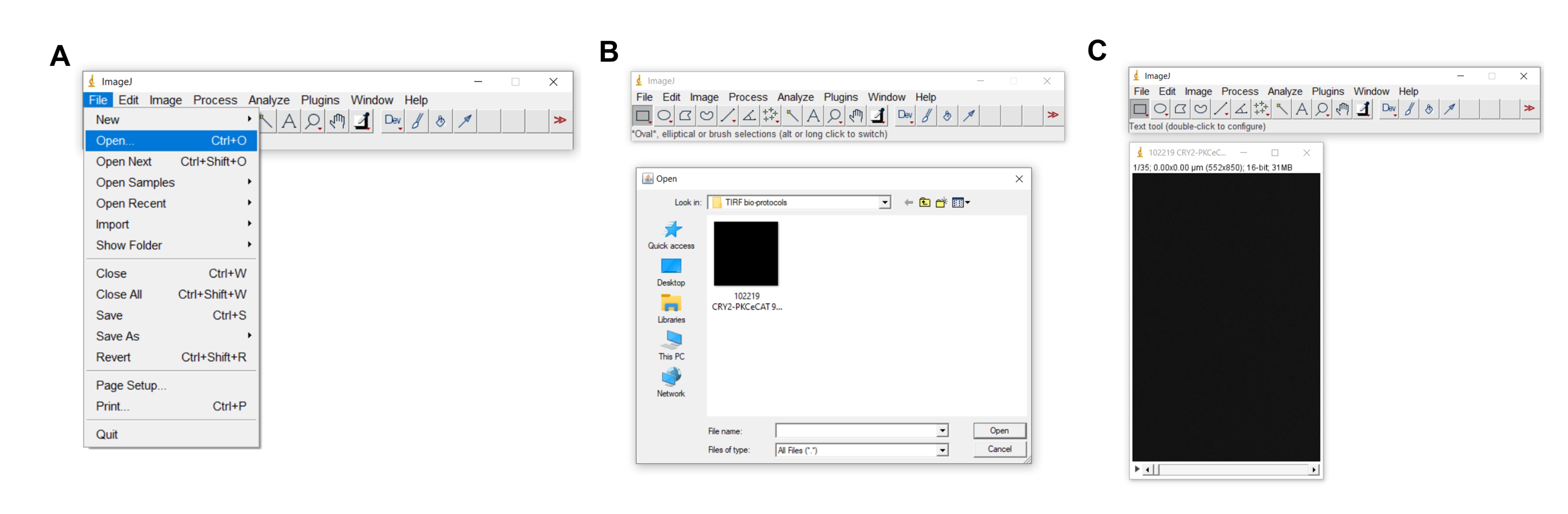
Figure 4. Launching TIF file in ImageJ. A–C depict how to launch (open) a TIF file in ImageJ.Click Image > Stacks > Tools > Make Substack (Figure 5)
In the area called “Slices,” number your slice. This will be your background slice from which all the slices are subtracted against. In the figure below, the slice is labeled “1.”
Save slice 1 as “tiff.”
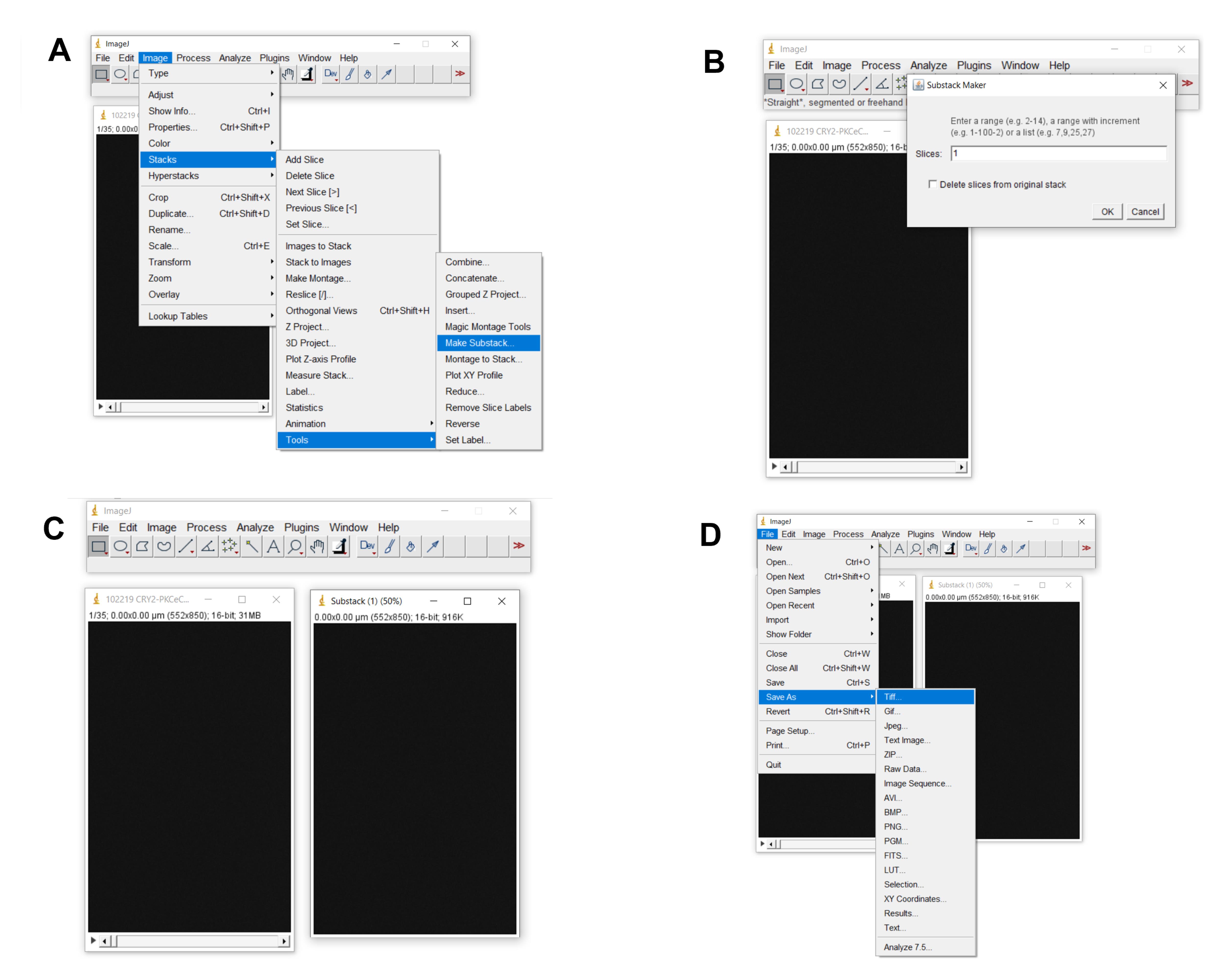
Figure 5. Creating and saving background/baseline slice. A and B. Depicts how to create a substack slice. C. The resulting file. D. Depicts how to save the substack file as a tiff.
Next click Process > Image Calculator (Figure 6)
Under “Image 1.”
Use the pull-down arrow to select the name of the file you are currently working on.
Under “Operation.”
Use the pull-down arrow to select the operation, “Subtract.”
Under “Image 2.”
Use the pull-down arrow to select the slice tiff image that you saved in the previous step.
Click OK.
A message will pop up asking if you want all the images to be processed; click “YES.”
A new window (results window) containing the processed images will pop up. Use this window moving forward.
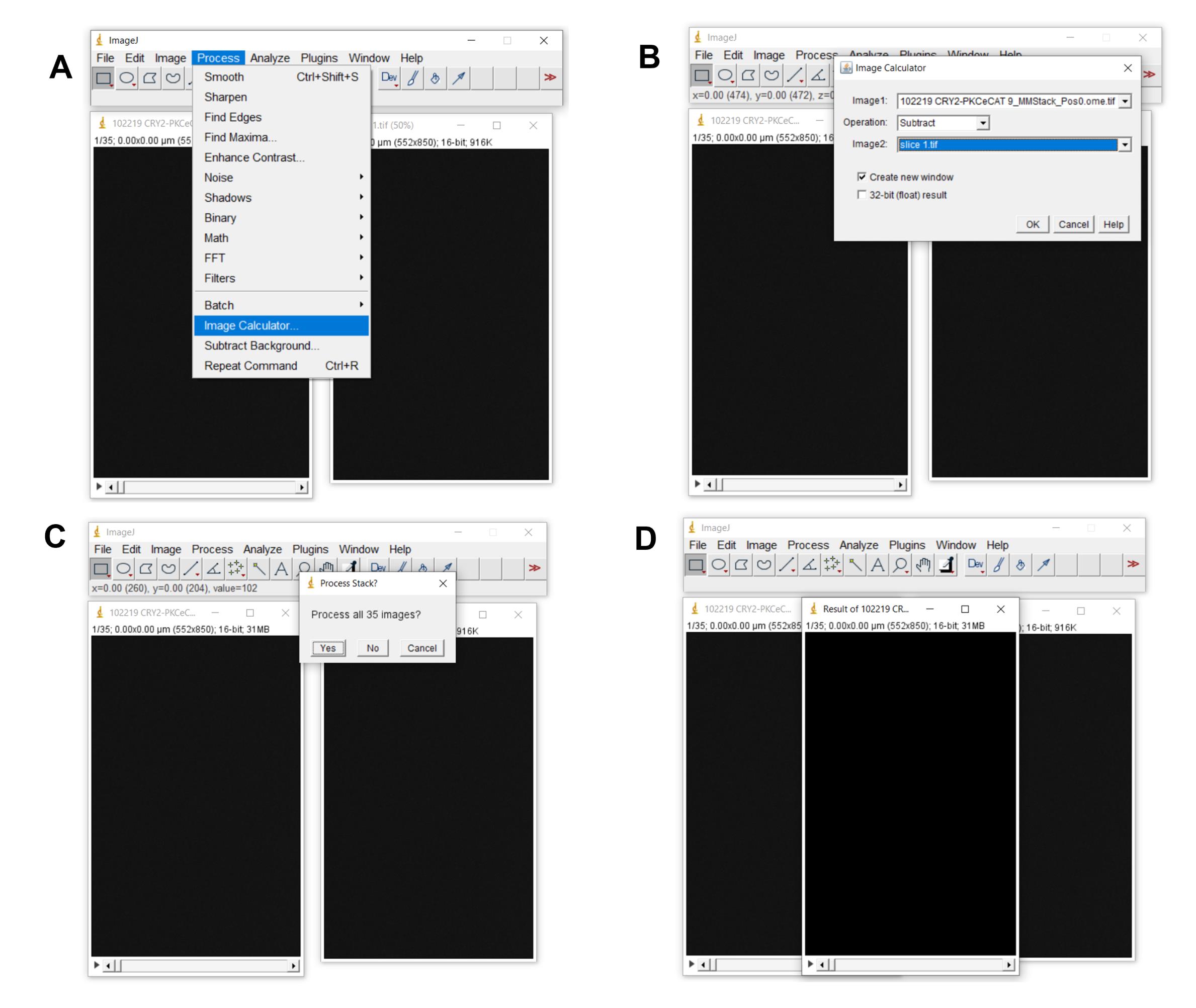
Figure 6. How to subtract background/baseline from all images/frames. A. Depicts how to launch image calculator to process images. B. Shows how image 2 (the slice file) is subtracted from the original file (Image 1). C. Depicts that all the images/frames are processed. D. The resulting file.
Click Image > Adjust > Brightness/contrast (Figure 7)
Scroll beyond the first few frames and then click auto. You should now be able to visualize your cell(s).
If you do not see your cell(s), scroll through a few more images and then click auto again. Do this until you can see the cell(s). Select the appropriate brightness and contrast that makes it possible to differentiate the cell(s) from the background.
Click apply.
Click OK when warned about pixel values changing.
When asked whether to apply to all slices, click “YES.”
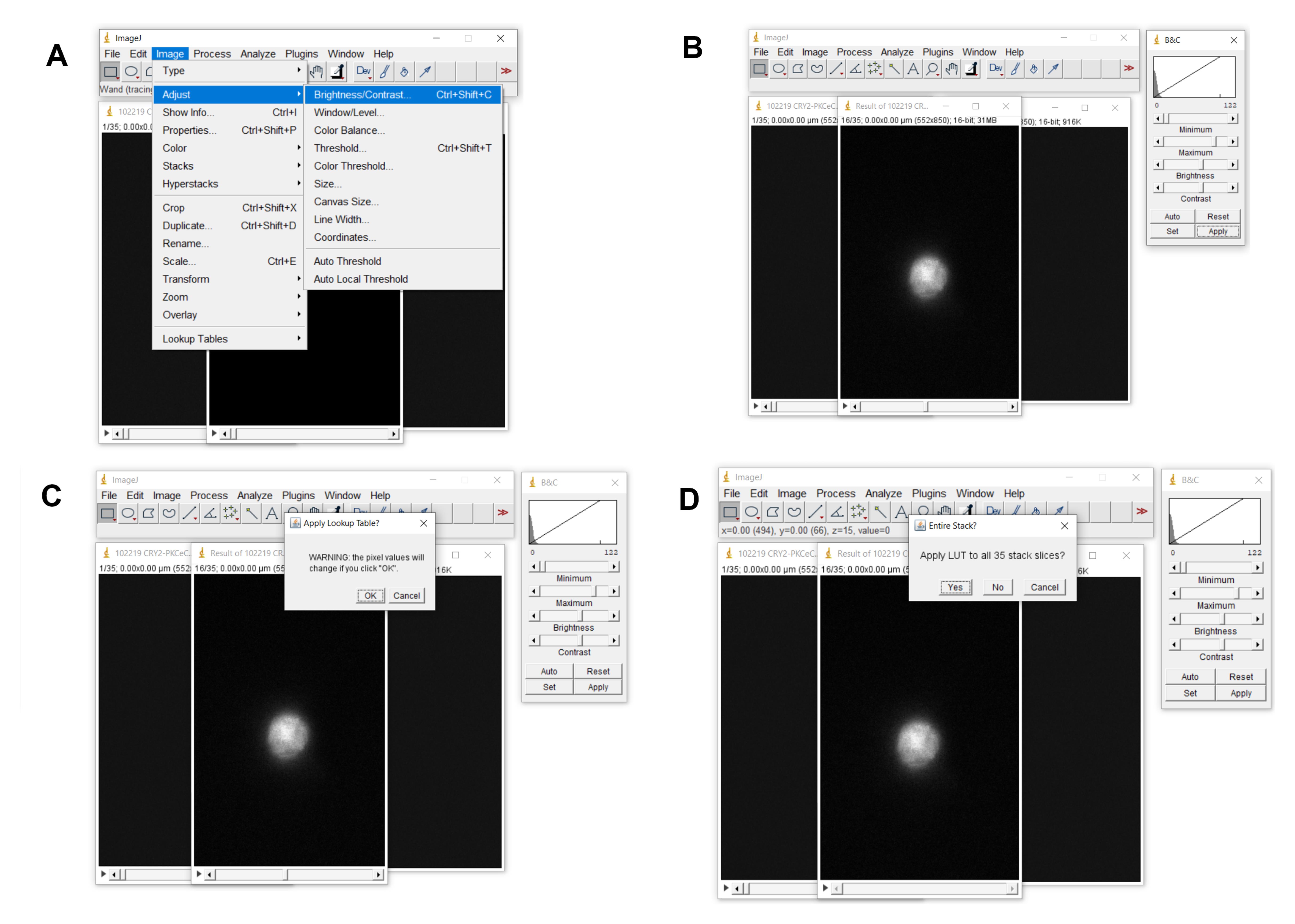
Figure 7. How to adjust brightness and contrast. A–D. Depicts how to adjust the brightness and contrast of the images.
Next click Analyze > Tools > ROI manager > Show all (Figure 8)
Select ROI on the image; then, click Add[t] (do this for each ROI added).
Once all your ROIs have been added, click More > Multi-Measure > OK.
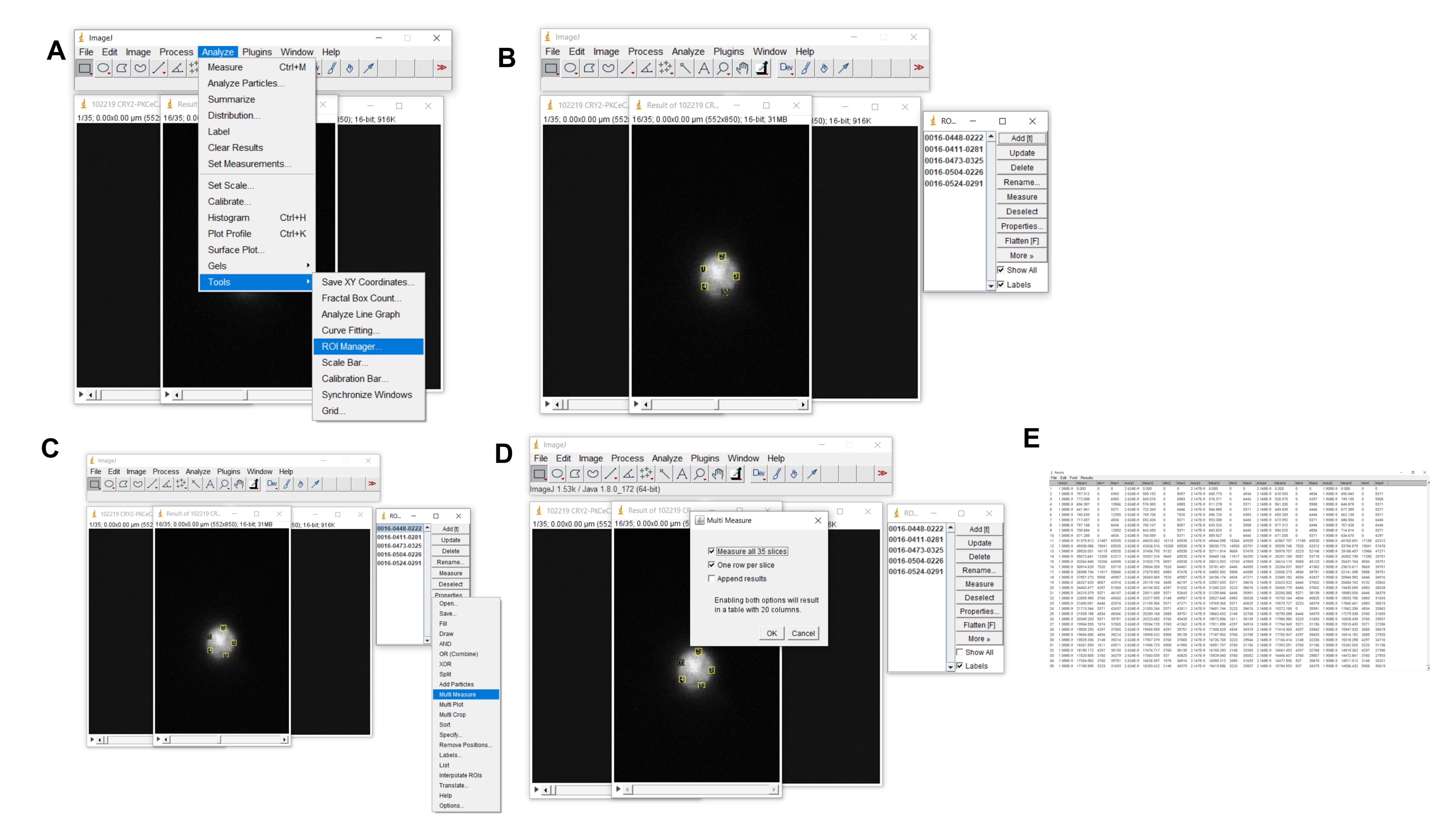
Figure 8. How to select and analyze region of interests (ROIs). A. Indicates how to launch region of interest (ROI) manager. B. Depicts five ROIs on the cell. Selected regions are indicated in the window to the right. C and D. Depicts how to launch multi-measure to measure ROIs across all images/frames. E. The resulting window with all the measurements.
Plot the mean fluorescence intensity vs. time to create a time course or to create summary bar graphs for various time points/treatments.
Include five or more cells in the analyses of each condition to create a summary graph with representative images and a time course of mean intensities, as well as a summary (Figure 9A and 8B respectively).
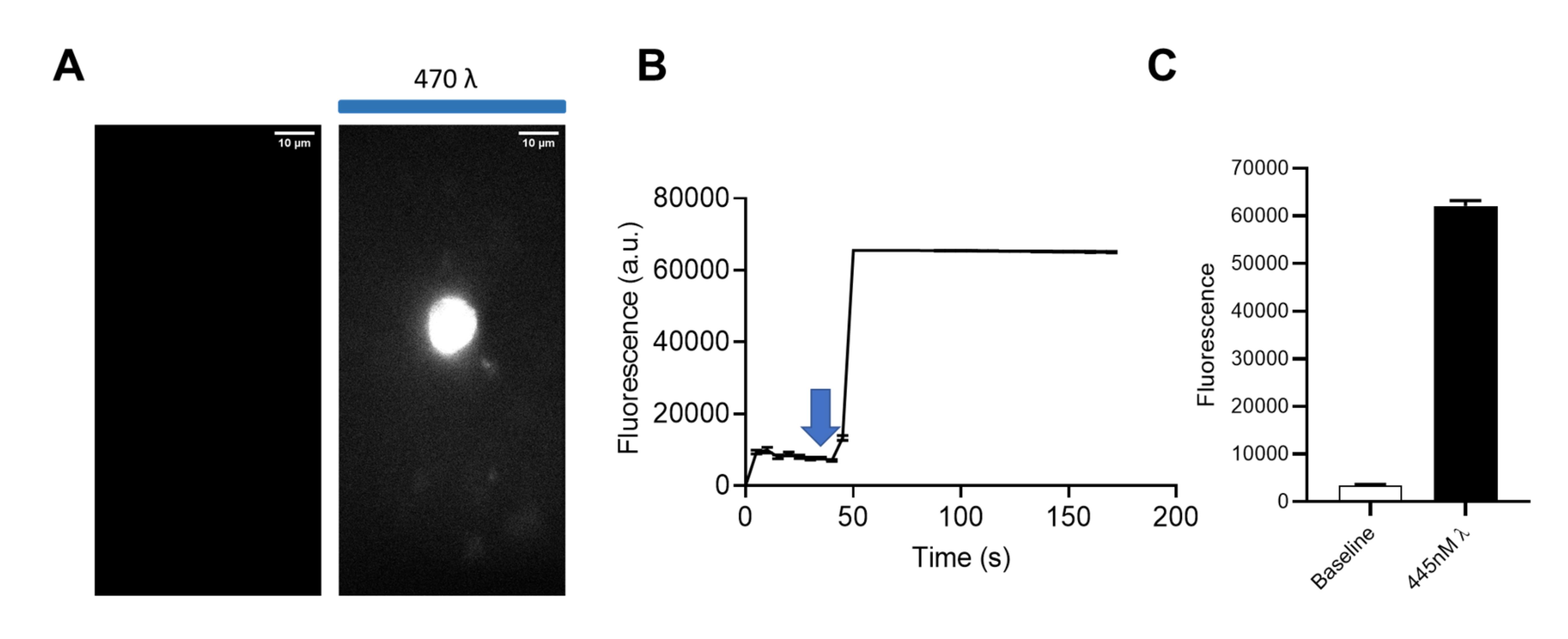
Figure 9. Final data representation. A. Representative images demonstrating fluorescence intensity before and after blue light activation of mCherry-CRY2-PKCϵCAT-HA. Scale bar = 10 µm. B. Time course of the experiment; blue arrow indicates the time point at which the 445λ laser was turned on. C. Summary data demonstrating the mean fluorescence intensity ± S.E. of 12 cells (Gada et al., 2022).
Recipes
TIRF imaging Solution
NaCl 130 mM
KCl 4 mM
MgCl2 1.2 mM
CaCl2 2 mM
HEPES 10 mM
Adjust pH to 7.4 with NaOH.
Acknowledgments
We thank Dr. Pietro De Camilli for providing CIBN-CAAX and CRY2-5’ptaseOCRL (Idevall-Hagren et al., 2012). This work was funded by National Institutes of Health Heart, Lung and Blood Institute grant R01HL144615 to L.D.P. This protocol was validated in Gada et al. (2022).
Competing interests
The authors declare that they have no competing interests with the contents of this article.
References
- Axelrod, D. (2001). Total internal reflection fluorescence microscopy in cell biology. Traffic 2(11): 764-774.
- Gada, K. D., Kawano, T., Plant, L. D. and Logothetis, D. E. (2022). An optogenetic tool to recruit individual PKC isozymes to the cell surface and promote specific phosphorylation of membrane proteins. J Biol Chem 298(5): 101893.
- Idevall-Hagren, O., Dickson, E. J., Hille, B., Toomre, D. K. and De Camilli, P. (2012). Optogenetic control of phosphoinositide metabolism. Proc Natl Acad Sci U S A 109(35): E2316-2323.
- Larson, J., Kirk, M., Drier, E. A., O'Brien, W., MacKay, J. F., Friedman, L. J. and Hoskins, A. A. (2014). Design and construction of a multiwavelength, micromirror total internal reflectance fluorescence microscope. Nat Protoc 9(10): 2317-2328.
- Liu, H., Yu, X., Li, K., Klejnot, J., Yang, H., Lisiero, D. and Lin, C. (2008). Photoexcited CRY2 interacts with CIB1 to regulate transcription and floral initiation in Arabidopsis. Science 322(5907): 1535-1539.
- Vangindertael, J., Camacho, R., Sempels, W., Mizuno, H., Dedecker, P. and Janssen, K. P. F. (2018). An introduction to optical super-resolution microscopy for the adventurous biologist. Methods Appl Fluoresc 6(2): 022003.
- Zong, W., Wu, R., Li, M., Hu, Y., Li, Y., Li, J., Rong, H., Wu, H., Xu, Y., Lu, Y., et al. (2017). Fast high-resolution miniature two-photon microscopy for brain imaging in freely behaving mice. Nat Methods 14(7): 713-719.
Article Information
Copyright
© 2023 The Author(s); This is an open access article under the CC BY-NC license (https://creativecommons.org/licenses/by-nc/4.0/).
How to cite
Readers should cite both the Bio-protocol article and the original research article where this protocol was used:
- Gada, K. D., Kamuene, J. M., Kawano, T. and Plant, L. D. (2023). Imaging Membrane Proteins Using Total Internal Reflection Fluorescence Microscopy (TIRFM) in Mammalian Cells. Bio-protocol 13(4): e4614. DOI: 10.21769/BioProtoc.4614.
- Gada, K. D., Kawano, T., Plant, L. D. and Logothetis, D. E. (2022). An optogenetic tool to recruit individual PKC isozymes to the cell surface and promote specific phosphorylation of membrane proteins. J Biol Chem 298(5): 101893.
Category
Biophysics > Microscopy
Cell Biology > Cell signaling > Phosphorylation
Cell Biology > Cell imaging > Fluorescence
Do you have any questions about this protocol?
Post your question to gather feedback from the community. We will also invite the authors of this article to respond.