Rapid Multiplexed Flow Cytometric Validation of CRISPRi sgRNAs in Tissue Culture

Materials and Reagents

1. 0.2 mL PCR tubes (USA Scientific, catalog number: 1402-2900)

2. Sterilized, low retention, LTS pipette tips (Rainin, catalog numbers: 30389213, 30389240, 30389226)

3. 1.5 mL Eppendorf Safe-Lock centrifuge tubes (USA Scientific, catalog number: 4036-3204)

4. Falcon 15 mL conical centrifuge tubes (Corning catalog number: 352097)

5. Falcon 50 mL conical centrifuge tubes (Corning, catalog number: 352098)

6. Accutec razor blades (ThermoFisher Scientific, catalog number: S17302)

7. 14 mL culture tubes (Avantor/VWR, catalog number: 60818-689)

8. Parafilm (ThermoFisher Scientific, catalog number: S37440)

9. 96-well, cell culture-treated, flat-bottom microplate (Corning, catalog number: 3903)

10. 5 mL, 10 mL, 25 mL, and 50 mL serologic pipettes (Santa Cruz Biotechnology, catalog numbers: sc-200279, sc-200281, sc-200283, sc-213234)

11. Countess cell counting chamber slides (ThermoFisher Scientific, catalog number: C10228)

12. Sterile 96-well v-bottom polypropylene plates (Corning, catalog number: 3357)

13. 50 mL, 250 mL, 500 mL, and 1000 mL Nalgene Rapid-Flow sterile single use vacuum filter units (ThermoFisher Scientific, catalog numbers: 5640020, 5680020, 5660020, 5670020)

14. 23G sterile blunt needles (ThermoFisher Scientific, catalog number: NC9031029)

15. NORM-JECT luer lock sterile syringes (Avantor/VWR, catalog number: 53548-023)

16. 90 micron nylon mesh (Elko Filtering, catalog number: 03-90/49)

17. Polypropylene microtiter (“bullet”) tubes (ThermoFisher Scientific, catalog number: 02-681-376)

18. 5 mL round bottom polystyrene with cell strainer cap (Corning, catalog number: 352235)

19. MultiScreenHTS HV sterile filter plate, 0.45 µm (Millipore Sigma, catalog number: MSHVS4510)

20. Aluminum foil (Avantor/VWR, catalog number: 89125-940)

21. Desalted, custom synthesized oligonucleotides (see step A1)

22. pCRISPRi/a v2 [Addgene, catalog number: 84832, and described in Horlbeck et al. (2016), store at -20°C]

23. FastDigest BstXI (ThermoFisher Scientific, catalog number: FD1024, store at -20°C)

24. FastDigest Bpu1102I/BlpI (ThermoFisher Scientific, catalog number: FD0094, store at -20°C)

25. Agarose LE (Goldbio, catalog number: A-201-100)

26. SYBR Safe DNA gel stain (ThermoFisher Scientific, catalog number: S33102)

27. E.Z.N.A. gel extraction kit (Omega Bio-Tek, catalog number: D2500-02)

28. E.Z.N.A. plasmid DNA mini kit I (Omega Bio-Tek, catalog number: D6942-02, some components of kit require storage at 4°C)

29. Isopropanol (Millipore Sigma, catalog number: 59304)

30. 1 kb DNA ladder (Goldbio, catalog number: D010-500, store long-term at -20°C, short-term at R.T.)

31. KOPTEC absolute ethanol (Avantor/VWR, catalog number: 89125-172)

32. Sodium acetate (Millipore Sigma, catalog number: S2889)

33. TempPlate non-skirted 96-well PCR plate, 0.2 mL (USA Scientific, catalog number: 1402-9596)

34. Adhesive PCR plate foil seals (Avantor/VWR, catalog number: 60941-076)

35. Potassium acetate (Millipore Sigma, catalog number: P1190)

36. HEPES (Goldbio, catalog number: H-400-100)

37. Tris base (Goldbio, catalog number: T-400-500)

38. Concentrated hydrochloric acid (Avantor/VWR, catalog number: JT9535)

39. Potassium hydroxide (Millipore Sigma, catalog number: P5958)

40. Magnesium acetate (Millipore Sigma, catalog number: M5661)

41. T4 DNA Ligase (New England BioLabs, catalog number: M0202L, store both enzyme and buffer at -20°C)

42. One Shot Mach1 T1 phage-resistant chemical competent E. coli (ThermoFisher Scientific, catalog number: C862003, store at -80°C)

43. Mix & Go! E. coli transformation kit (Zymo Research, catalog number: T3001, some components of kit require storage at 4°C)

44. LB Broth (Millipore Sigma, catalog number: L3522)

45. Carbenicillin (Goldbio, catalog number: C-103-5, store at -20°C)

46. LB-agar plates carbenicillin-100 (Teknova, catalog number: L1010, store at 4°C)

47. Zyppy-96 plasmid kit (Zymo Research, catalog number: D4042, some components of kit require storage at 4°C)

48. Lab markers (ThermoFisher Scientific, catalog number: 13-379-4)

49. Glycerol (Millipore Sigma, catalog number: G2025)

50. HEK-293T cells (ATCC, catalog number: CRL-3126, store at -80 to -150°C)

51. Gibco high-glucose DMEM with pyruvate and GlutaMax supplement (ThermoFisher Scientific, catalog number: 10569010, store at 4°C protected from light)

52. Gibco low-glucose DMEM with pyruvate and GlutaMax supplement (ThermoFisher Scientific, catalog number: 10567014, store at 4°C protected from light)

53. Heat-inactivated fetal bovine serum (FBS) (Axenia Biologix, catalog number: F002, aliquot and store at -20°C)

54. Lipoprotein depleted FBS (Kalen Biomedical, catalog number: 880100, aliquot and store at -20°C)

55. Human 3,3’-dioctadcylindocarbocyanine low density lipoprotein (DiI-LDL) (Kalen Biomedical, catalog number: 770230-9, store at 4°C protected from light)

56. Clorox bleach (Office Depot, catalog number: 217595)

57. Lentiviral packaging vectors: pCMV-dR8.91 and pMD2.G (Addgene, catalog number: 12259, and described in (Gilbert et al., 2014), store at -20°C)

58. ViralBoost reagent (Alstem, catalog number: VB100, store at 4°C)

59. Opti-MEM I reduced serum medium (ThermoFisher Scientific, catalog number: 31985062, store at 4°C protected from light)

60. TransIT-LT1 transfection reagent (Mirus Bio, catalog number: MIR2300, store at 4°C)

61. Puromycin (Invivogen, catalog number: ant-pr-1, store at -20°C)

62. Bovine serum albumin (Millipore Sigma, catalog number: 12659, store at 4°C)

63. Sterile reagent reservoirs (Corning, catalog number: 4870)

64. Polybrene infection/transfection reagent (ThermoFisher Scientific, catalog number: TR-1003-G, store at -20°C))

65. Trypsin-EDTA (0.25%) with phenol red (ThermoFisher Scientific, catalog number: 25-200-114, store long-term at -20°C, short-term at 4°C)

66. Phosphate buffered saline (PBS), pH 7.4, sterile (ThermoFisher Scientific, catalog number: 10010049)

67. Accutase (Innovative Cell Technologies, catalog number: AT104, store long-term at -20°C, short-term at 4°C)

68. Gibco 100× penicillin-streptomycin (ThermoFisher Scientific, catalog number: 15140122, store long-term at -20°C, short-term at 4°C)

69. DNase I (Goldbio, catalog number: D-300-100, store at -20°C)

70. CRISPRi-ready cells (dCas9-BFP-KRAB HepG2 cells are described in (Smith et al., 2022), store at -80 to -150°C)

71. Ghost Dye red 780 (Tonbo Biosciences, catalog number: 13-0865-T100, store at -20°C)

72. Human LDLR Alexa Fluor 647-conjugated antibody (R&D Systems, catalog number: FAB2148R, store at 4°C)

73. Human TfR Alexa Fluor 488-conjugated antibody (R&D Systems, catalog number: FAB2474G, store at 4°C)

74. Dimethyl sulfoxide (Millipore Sigma, catalog number: D2650)

75. 16% formaldehyde solution (Avantor/VWR, catalog number: 100503-917)

76. 2× Annealing Buffer (see Recipes)

77. 50× TAE Buffer (see Recipes)

78. 293T growth medium (see Recipes)

79. Viral harvest medium (see Recipes)

80. HepG2 growth medium (see Recipes)

81. Sterol-depleted medium (see Recipes)

82. FACS buffer (FB) (see Recipes)

83. DiI-LDL labeling medium (see Recipes)

Equipment

1. 2 µL, 20 µL, 200 µL, and 1000 µL LTS Pipet-Lite XLS+ manual single channel pipettes (Rainin, catalog number: 30386597)

2. 10 µL, 20 µL, and 200 µL Pipet-Lite XLS+ manual 12-channel pipettes (Rainin, catalog numbers: 17013807, 17013808, 17013810)

3. Pipet-Aid XP2 (USA Scientific, catalog number: 4440-5010)

4. Milli-Q Direct 16 water purification system (Millipore Sigma, catalog number: ZR0Q016WW)

5. ProFlex 3 × 32 well PCR thermocycler (ThermoFisher Scientific, catalog number: 4484073)

6. Mini-Sub Cell GT horizontal electrophoresis system and PowerPac basic power supply (Bio-Rad, catalog number: 1640300)

7. E-Gel imager system with blue-light base (ThermoFisher Scientific, catalog number: 4466612)

8. Dry block heater with 1.5 mL microcentrifuge tube block (Avantor/VWR, catalog numbers: 75838-318, 13259-286)

9. QIAVac 24 Plus vacuum manifold (Qiagen, catalog number: 19413)

10. Microcentrifuge (Eppendorf, catalog number: 5425)

11. NanoDrop 2000 UV-Vis spectrophotometer (ThermoFisher Scientific, catalog number: ND-2000)

12. Heratherm compact microbiological incubator (ThermoFisher Scientific, catalog number: 50125590)

13. New Brunswick Innova 44R incubator shaker (Eppendorf, catalog number: M12820006)

14. Binder CO₂ incubator (Avantor/VWR, catalog number: CB170)

15. Vortex mixer (Avantor/VWR, catalog number: 10153-838)

16. FiveEasy pH meter (Mettler Toledo, catalog number: 30266626)

17. -20°C laboratory freezer (ThermoFisher Scientific, catalog number: 02LFEETSA)

18. Ice buckets (Avantor/VWR, catalog number: 10146-188)

19. Allegra X-30R benchtop centrifuge with SX4400 and S606 rotors (Beckman Coulter, catalog number: B06320)

20. Scotsman FLAKER ice maker (CurranTaylor, catalog number: SCF1415A)

21. Aluminum alloy cooling block for 0.2 mL PCR tubes (ThermoFisher Scientific, catalog number: 13-131-013)

22. Laboratory refrigerator (ThermoFisher Scientific, catalog number: TSG25RPGA)

23. Ultra low temperature freezer (ThermoFisher Scientific, Forma catalog number: 995)

24. Countess II FL automated cell counter (ThermoFisher Scientific, catalog number: A32136)

25. Flow cytometer, such as: LSRFortessa with HTS sampler (BD Biosciences), LSRII (BD Biosciences), or CytoFLEX (Beckman Coulter)

26. Autoclave machine

27. Tissue culture hood

28. Laboratory microscope (for tissue culture)

29. Chemical fume hood

Software

1. ApE, A plasmid Editor [Described in Davis and Jorgensen (2022) https://jorgensen.biology.utah.edu/wayned/ape/]

2. Flow cytometer acquisition software: FACSDiva (BD Biosciences, https://www.bdbiosciences.com/en-us/products/software/instrument-software/bd-facsdiva-software) or CytExpert (Beckman Coulter, https://www.beckman.com/flow-cytometry/research-flow-cytometers/cytoflex/software)

3. Prism (GraphPad, https://www.graphpad.com)

4. FlowJo (BD Biosciences, https://www.flowjo.com)

5. Excel (Microsoft, https://www.microsoft.com/en-us/microsoft-365/excel)

Procedure

Pre-requisite: Perform primary CRISPRi/a screen and identify hits for further validation.

1. Cloning of Validation sgRNA Lentiviral Vectors

   Note: This cloning protocol has been modified from resources at https://weissman.wi.mit.edu/crispr/, and is reproduced here for convenience.

   1. Oligonucleotide Design

      1. Use the following template to order standard de-salted oligonucleotides from a vendor of choice, pre-suspended at 100 µM concentration, with one pair (“top” and “bottom”) for each sgRNA to test. The oligos are designed to anneal into a double digest of BstXI and BlpI (Figure 1).

         
         

         sgRNA	Template	LDLR 1 (Example)
         Protospacer(20 nt)	N1,N2 …N20	GTTACCTGCAGTCCCCGCCG
         “Top” Oligo(33 nt)	ttg(N1,N2 …N20 )gtttaagagc	ttgGTTACCTGCAGTCCCCGCCGgtttaagagc
         “Bottom” Oligo(40 nt)	ttagctcttaaac(R.C. of N1,N2 …N20)caacaag	ttagctcttaaacCGGCGGGGACTGCAGGTAACcaacaag

         R.C. = reverse complement

         
         

         
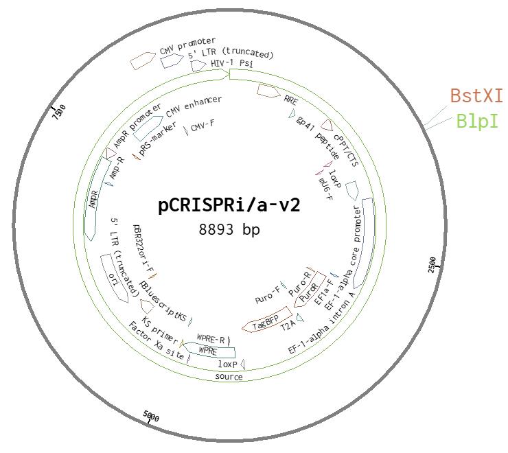
         Figure 1. Vector Map of pCRISPRi/a-v2. The cleavage sites for BlpI and BstXI are highlighted.

         
         

      2. Order separate 96-well plates for the “Top” and “Bottom” oligonucleotides, arraying the pair in the matched wells of the complementary plates.

         Note: The orientation of sgRNAs target in this plate can then be carried forward throughout the entire protocol. Multiple control sgRNAs should be included for the final phenotypic experiment, including those expected to produce a phenotypic effect (biologic controls) and those expected to have a null effect (non-targeting controls). Including non-targeting controls in the last well of every row on a 96-well plate allows for eight biological replicates per plate (Figure 2).

         
         

      
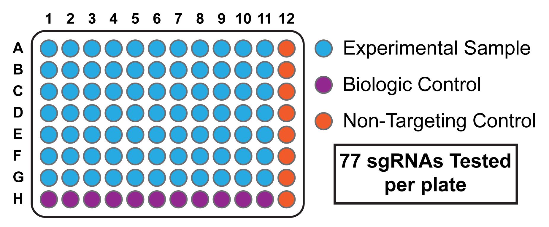
      Figure 2. Sample Layout of 96-well Plate. Each experimental sample corresponds to a unique sgRNA, with space reserved for biological controls (sgRNAs expected to produce either a gain or loss of function) and non-targeting controls (sgRNAs expected to have a null effect). After a genome-wide screen, typically two sgRNAs are validated per gene.

      
      

   2. Vector Digestion

      1. Combine the following reagents in a PCR tube. Set up separate tubes for each 5-µg vector digest required.

         Reagent	Amount
         10× FastDigest Green Buffer	5 µL
         pCRISPRi/a-v2	5 µg
         BlpI	2.5 µL
         BstXI	2.5 µL
         Milli-Q H2O	to 50 µL total

         Note: 5 µg of purified, digested vector is required for each 96-well plate of sgRNAs to be obtained.

         
         

      2. Incubate reaction in a PCR thermocycler at 37°C for 1 h.

      3. Heat inactivate the reaction at 80°C for 10 min.

      4. Resolve entire digest over a 0.7% agarose gel run in TAE buffer, visualize, and excise the band containing the linearized vector. Gel purify the excised band using a gel purification kit, according to the manufacturer’s instructions.

      5. Quantify the concentration of purified, digested vector using NanoDrop UV-Vis spectrophotometer.

   3. Oligonucleotide Annealing

      1. Combine the following components in a fresh 96-well PCR plate, using a multichannel pipette:

         Reagent	Amount
         2× Annealing Buffer	20 µL
         Top Oligo (100 µM)	0.8 µL
         Bottom Oligo (100 µM)	0.8 µL
         Milli-Q H2O	18.4 µL
         Total Volume	40 µL

         
         

      2. Incubate the reaction in a PCR thermocycler at 95°C for 5 min.

      3. Remove the plate from the thermocycler while still at 95°C and allow to cool to room temperature (RT) on the benchtop for 15 min.

      4. Dilute 1 µL of annealed oligonucleotide mixture in 19 µL of Milli-Q H₂O, in a fresh 96-well PCR plate.

      Note: Annealed oligonucleotides can be stored at -20°C.

   4. Ligation

      1. Create ligation master mixes for each 96-well plate of ligations, as indicated below:

         Note: Creation of two master mixes allows the T4 DNA ligase to be kept separate from the digested vector until in the presence of the oligonucleotide insert, reducing self-ligation.

         Reagent	Final Amount (per well)	MM1 (per 96-well plate)	MM2 (per 96-well plate)
         10× T4 Ligase Buffer (fresh)	1×	60 µL	40 µL
         Digested pCRISPRi/a-v2 vector	50 ng	5 µg	-
         T4 Ligase	0.5 µL	-	50 µL
         Milli-Q H2O	to 10 µL	to 500 µL	310 µL
         Total Volume	10 µL	500 µL	400 µL

         
         

      2. To each well of a 96-well PCR plate placed on ice, aliquot 5 µL of ligation MM₁ , then 1 µL of diluted annealed oligonucleotide mixture, then 4 µL of ligation MM₂ .

      3. Seal the top of the plate, and incubate at 16°C overnight.

      4. Optional : After incubation, heat inactivate the T4 ligase at 65°C for 10 min.

   5. Transformation

      1. On ice, aliquot 10 µL of competent Mix & Go! Mach1 E. coli cells to each well of a 96-well plate.

         Note: Competent E. coli can be obtained direct from the vendor, or can be made competent using the Mix & Go! transformation kit, according to the manufacturer’s instructions. Competent cells will quickly lose competency if warmed, so pipette quickly. Pre-chilling the receiver plate and pipette tips to 4°C can also improve the yield of transformants.

      2. Add 1 µL of each ligation reaction to the competent cells. Incubate on ice for 30 min.

      3. Optional if using Mix & Go! cells : Heat shock the cells in the 96-well plate in a PCR thermocycler at 42°C for 45 sec, then immediately return to ice for 2 min.

      4. Partition LB-carbenicillin agar plates into 12 segments. Eight plates will be required for each 96-well plate of sgRNAs.

      5. Spot 5 µL of competent cells at the edge and streak towards the center of the plate with a pipette tip (Figure 3).

         
         

         
         Figure 3. Partitioned LB Agar Plate. Each LB agar plate is split into 12 segments. The transformed mixture is spotted at the edge, and then streaked within the partition, to allow for the selection of individual clones. Streaking within the partitioned area will reduce the risk of contamination between plasmids.

         
         

      6. Incubate plates at 37°C overnight, to allow for colony growth.

         Note: Avoid prolonged incubations, as very large colony sizes will make it difficult to select clones and increase the risk of cross-contamination.

   6. Clonal Plasmid Isolation

      1. Inoculate each well of a 96-well culture block from a Zyppy-96 Plasmid kit containing 760 µL of LB-carbenicillin (at 100 µg/mL) with a colony from each sgRNA-encoding plasmid. Store culture plates at 4°C after colony picking.

         Note: Selecting two clones per sgRNA for small scale culture growth, each in the corresponding well of separate 96-well-blocks, will improve the chance of obtaining the desired sgRNA sequence.

      2. Seal the plate with an air-permeable cover according to the manufacturer’s instructions, and incubate in a shaker at 220–300 rpm and 37°C overnight (12–18 h).

      3. After overnight growth, make glycerol stocks for convenient regrowth of plasmids. Transfer 10 µL of each culture into 10 µL of sterile 50% glycerol (in H₂O) in a PCR plate. Cover with a plate cover, and store at -80°C.

      4. Isolate plasmids from cultures in 96-well blocks using a Zyppy-96 kit, according to the manufacturer’s instructions.

      5. Determine concentration and purity of isolated plasmids using a NanoDrop spectrophotometer.

      6. Submit samples for Sanger sequencing to a vendor of choice. The following oligonucleotide can be used as the sequencing primer to read out the final protospacer sequence for each clone:

         5′-CGCCAATTCTGCAGACAAA-3′.

      7. Align sequences using sequence alignment software (ApE), and determine which colonies have the correct sgRNA sequence.

      8. For sgRNAs where neither selected clone has the correct sequence, grow four additional small-scale (i.e., 2–5 mL) cultures overnight selected from individual colonies on the stored culture plates, and then purify plasmids using a standard Mini-Prep procedure, and confirm the correct sequencing by Sanger sequencing.

      9. After all desired plasmids are obtained, create a master array of the sgRNA delivery plasmids in a fresh 96-well plate in a sterile tissue culture hood. Normalize plasmid concentrations to 25 ng/µL with either Milli-Q H₂O or elution buffer. Seal the plate, and store at -20°C.

         Note: This array offers an opportunity to re-orient the sgRNAs in the 96-well plate, if desired.

         
         

2. Lentiviral Production

   1. The day prior to transfection, seed HEK-293T cells in tissue culture treated 96-well plates in 100 µL of growth media (high-glucose DMEM with 10% FBS) at 2.2 × 10⁴ cells per well. Grow in 5% CO₂ at 37°C overnight.

      Note: Aim for cells to be 70%–80% confluent at time of transfection. To optimize viral production, use low-passage HEK-293T cells that have not previously grown to over-confluence. Confirm that cells appear morphologically normal prior to transfection.

   2. On the day of transfection, prepare the DNA and transfection reagent in sterile 96-well V-bottom plates in the tissue culture hood, as follows:

      1. Aliquot 4 µL of each normalized sgRNA vector (100 ng) to a sterile 96-well plate using a multichannel pipette.

      2. Make separate master mixes of packaging and envelope plasmids, and diluted transfection reagent, in OptiMEM, as indicated. Add the transfection reagent to OptiMEM dropwise, and mix by gently flicking the tube. Allow the diluted transfection reagent to incubate at RT for 5 min.

         Reagent	Final Amount (per well)	MM1 (for 120 wells)	MM2 (for 120 wells)
         pCMV-dR8.91	90 ng	10.8 µg	-
         pMD2.G	11 ng	1.32 µg	-
         Trans-LT1	0.6 µL	-	72
         Opti-MEM	to 14 µL	to 600 µL	528 µL
         Total Volume	14 µL	600 µL	600 µL

         
         

      3. Briefly vortex plasmid mix, and aliquot 5 µL of this to each well of the plate using a multichannel pipette.

      4. Aliquot 5 µL of diluted transfection reagent to each well of the plate. Briefly, mix by tapping the side of the plate. Cover the top of the plate, and incubate at RT for 30 min.

      5. Using a multichannel pipette, transfer all 14 µL of transfection mix to the corresponding wells of previously seeded plate(s) of HEK-293T cells.

      6. Incubate cells at 5% CO₂ and 37°C for 6–8 h.

      7. Carefully remove transfection mixture and growth media from each well. Carefully replace with 100 µL of viral harvest medium (growth medium with 11 g/L BSA) supplemented with 1× ViralBoost (0.2 µL 500× ViralBoost per 100 µL medium).

         Note: Tilt plate and position tip at bottom of the well to avoid aspirating cells. Slowly pipette replacement media along the side of well to avoid dislodging cells .

      8. Return plate to incubator at 5% CO₂ and 37°C.

      9. Forty-eight hours after transfection, add another 100 µL of fresh viral harvest medium containing 1× ViralBoost to each well.

      10. Optional : If viral yields prove inadequate, a double harvest can be performed: the viral-containing media can be removed and replaced with 100 µL of fresh viral harvest media (with ViralBoost), with the conditioned media stored at 4°C, to be pooled with the subsequent harvest.

          Note: Decontaminate all tips in contact with virus with 10% bleach solution. Keeping a small container of bleach in the hood is a convenient way to dispose of tips, and collect discarded virus-containing liquids.

   3. Harvest virus-containing supernatant 68–72 h after transfection:

      1. Transfer media to sterile MultiScreenHTS filter plates, centrifuge at 500 × g for 1 min, and recover the virus-containing filtrate. Cover the plate and store at 4°C for short-term use (within 24 h); otherwise, store at -80°C.

         Note: Timing the transduction of the CRISPRi/a-ready cells to coincide with the day of the final harvest allows transduction with the highest possible viral titer. Formally titering the lentivirus is generally not required, and the virus-containing supernatant can be used directly for transductions.

      2. Optional : If filter plates are unavailable, the media can be transferred to a sterile 96-well V-bottom plate, and centrifuged at 1,250 × g for 5 min to pellet residual cells or debris. The resulting supernatant can be transferred to a fresh plate for storage.

         Note: This procedure can be easily scaled to transfect more than one 96-well plate of HEK-293T cells for each sgRNA, if greater volumes of viral supernatant are required.

         
         

3. Transduction of CRISPRi/a-ready Cells

   Note: CRISPRi (dCas9-BFP-KRAB) HepG2 cells are used in this protocol, but any adherent CRISPRi/a-ready cell line should be amenable to this procedure. To reduce clumping of HepG2 cells, which occurs over time, pass the cells through a 20–23G needle three times when passaging.

   1. On the day prior to transduction, seed CRISPRi/a-ready cells in 96-well plates in 100 µL of appropriate growth media. Aim for 50% confluence on day of transduction. For dCas9-BFP-KRAB HepG2 cells, seed 5 × 10⁴ cells per well in low-glucose DMEM with 10% FBS.

      Note: Seeding cell density will depend on the specific cell size and type.

   2. On day of transduction, add polybrene to a final concentration of 8 µg/mL per well, accounting for both the 100 µL of growth media and additional viral supernatants. Dilute 40 µL of the 10 mg/mL polybrene stock into 460 µL of sterile PBS, to obtain a 100× solution, and then aliquot 1.5–2 µL of this to each well.

   3. Add 50–100 µL of viral supernatants directly to each well.

   4. Optional: Spinfect the cells by centrifuging plates at 800 × g at RT for 60 min, to modestly increase transduction rates. If necessary to obtain adequate transduction, the media can be removed after spinfection, and replaced with fresh media and additional viral supernatant.

   5. Incubate cells with 5% CO₂ at 37°C for 48 h.

   6. Forty-eight hours after transduction, split cells 1:2 into a fresh 96-well plate:

      1. Remove media from each well, and wash cells with 100 µL of PBS.

      2. Dissociate the monolayer by adding 50 µL of 0.25% sterile Trypsin-EDTA solution. Incubate with 5% CO₂ at 37°C for 5–10 min.

      3. Quench trypsin by adding 150 µL of growth media. Fully suspend cells by pipetting up and down.

      4. Transfer 50% of each suspension (~95 µL) to a fresh tissue culture plate.

      5. Return plates to incubator with 5% CO₂ at 37°C.

      6. Optional : If cells are particularly sensitive to trypsin, consider quenching trypsin with 50 µL of growth media, transferring cells to a sterile 96-well V-bottom plate, and removing trypsin-containing supernatant after pelleting cells (500 × g for 5 min). Cells can then be resuspended and transferred to fresh tissue culture plates.

   7. Twenty-four hours after split, select for successful transduction with puromycin:

      1. Carefully remove the conditioned media on top of the cells.

      2. Replace with fresh growth media containing puromycin at a final concentration of 2 µg/mL.

      3. Return plates to incubator with 5% CO₂ at 37°C.

      Note: Puromycin selection should be omitted if the downstream phenotypic experiment will directly compare transduced vs non-transduced cells within the same well (this can be distinguished by TagBFP levels induced by the sgRNA-containing pCRISPRi/a-v2 vector). If puromycin is expected to result in an adverse phenotype, adding an excess of virus can assure a high percentage of transduced cells. In this case, to assess the transduction efficiency, a test well should be reserved for puromycin selection, either within the same plate or cultured in parallel.

   8. Forty-eight hours after puromycin selection, remove puromycin, and exchange cells into fresh growth media.

   9. Monitor cell growth and prepare cells for phenotypic experiments. As cells near confluency, split cells according to the procedure above.

      Note: At this stage, creating three “copies” of the plates is helpful: 1) a maintenance plate for propagation, 2) an experimental plate to perform the phenotypic experiment, and 3) a storage plate in freezing medium (growth medium with 10% DMSO) for long-term storage at -150°C.

      
      

4. Phenotyping of Cells: Receptor Labeling

   Note: Surface levels of the LDL and transferrin receptors are evaluated in this protocol, but labeling of any antibody-detectable cell surface marker should be feasible with this procedure. Select orthogonal fluorophores for receptor labeling, TagBFP levels, and live/dead staining within the detection capabilities of the flow cytometer available. For each plate, include one well for each single stained control and fluorescence minus one (FMO) control, and two wells for completely unstained controls. Parental (i.e., non-sgRNA-transduced) CRISPRi-ready cells can typically be used for these controls. Two additional fully stained controls (harboring control sgRNA) should also be included, to evaluate instrumental drift at the beginning and end of the flow cytometry. Each of these additional wells can be included either within the plate or cultured in parallel.

   1. Prepare experimental plate from part C as appropriate for the phenotypic experiment, and avoid over-confluency. For HepG2-derived cells, inducing sterol starvation upregulates LDL receptor abundance (Horton et al., 2002).

      Note: To increase throughput, trypsinize the experimental plate, and seed three daughter plates to perform the experiment in triplicate.

      1. Remove media from cells, wash with 100 µL of PBS, and replace with 75 µL of sterol-depleted media per well (low-glucose DMEM with 5% lipoprotein-deficient serum).

      2. Return plate to incubator with 5% CO₂ at 37°C, and incubate overnight.

   2. Harvest cells

      1. Remove media from cells, and wash with 100 µL of PBS.

      2. Add 40 µL of Accutase per well, and incubate the plate on an orbital shaker at RT for 15 min.

         Note: Accutase has no effect on the levels of either the LDL or transferrin receptors detected by antibody labeling when compared to non-enzymatic or physical dissociation methods. Confirm that this method of dissociation does not affect the surface protein/epitope of interest.

      3. Add 50 µL of FACS Buffer (PBS with 1% FBS and 10 U/mL DNase I) to each well, and pipette up and down vigorously to dissociate the cells.

      4. Filter cells through a 90-µm nylon mesh taped to the top of a V-bottom plate placed on ice (Figure 4).

         
         

         
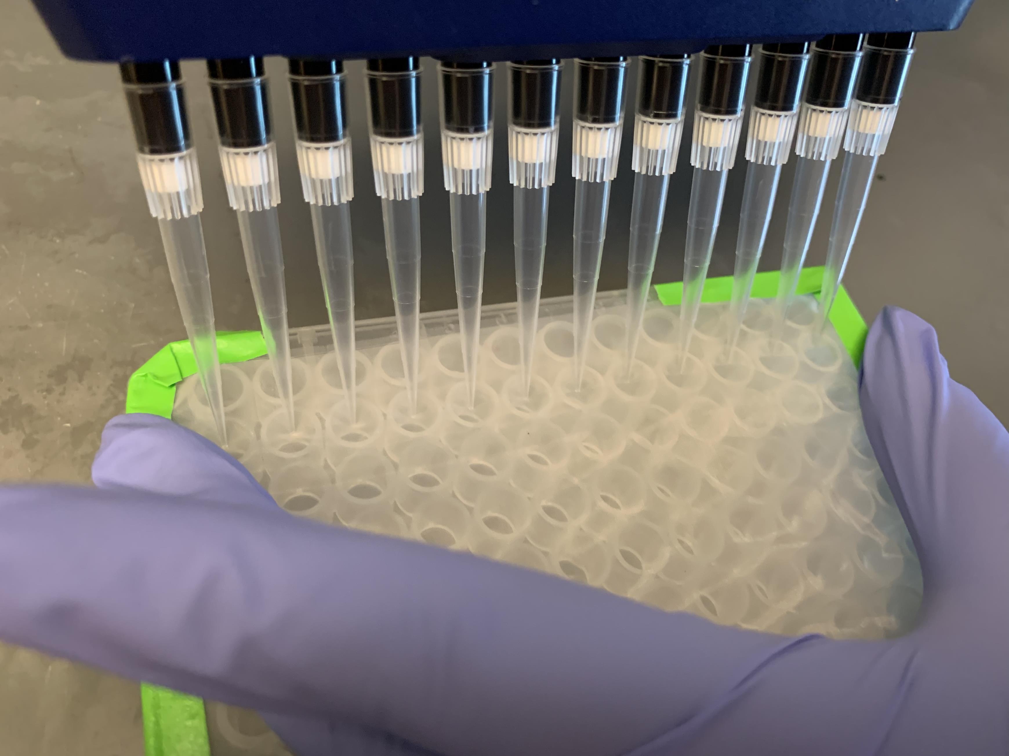
         Figure 4. Cell Filtration. Filtration is a key step to maximize singlets and prevent clogs during flow cytometry. Holding the sides of the mesh to keep it taut while pressing gently against the mesh with the pipette tips allows the liquid to travel through the mesh and into the wells. If the liquid accumulates on top of the mesh, it can mix with and contaminate neighboring wells.

         
         

      5. Centrifuge plate at 2,000 × g and 4°C for 1–2 min. Remove the mesh and discard the supernatant.

         Note: Invert the plate and give a quick but forceful downward shake to remove the supernatant. The cells will remain at the bottom of the wells.

      6. Wash the cells by resuspending them in 200 µL of FACS Buffer. Centrifuge the plate again at 2,000 × g and 4°C for 1–2 min, and discard the supernatant.

   3. Label cells with live/dead stain:

      1. Resuspend cells in 50 µL of a 1:1,000 dilution of Ghost Red 780 stain in PBS. Cover from light and incubate the plate on an orbital shaker on ice for 10 min. Retain one well each for a live-dead stain-negative control, additional wells for each single stained antibody control, and two wells for completely unstained controls – these wells should be resuspended in 50 µL of PBS.

         Note: The choice of live/dead stain depends on the fluorophores used for labeling.

      2. Add 200 µL of FACS Buffer, centrifuge the plate at 2,000 × g and 4°C for 1–2 min, and discard the supernatant.

      3. Wash the cells by resuspending them in 200 µL of FACS Buffer. Centrifuge the plate again at 2,000 × g and 4°C for 1–2 min, and discard the supernatant.

   4. Label cell surface receptors with appropriate fluorophore-conjugated antibodies:

      1. Resuspend cells in 40 µL of FACS buffer containing a 1:50 dilution of anti-LDLR-A647 and 1:100 dilution of anti-TFR-A488. Cover from light and incubate the plate on an orbital shaker on ice for 30–45 min. Retain one well for each single stained antibody control (LDLR and TFR), one well for each antibody negative FMO control (LDLR-negative and TFR-negative), and two wells for the completely unstained controls—these wells should be resuspended in FACS buffer containing a 1:50 dilution of anti-LDLR-A647, a 1:100 dilution of anti-TFR-A488, or no antibody, as appropriate.

         Note: The choice of antibody and fluorophore depends on the experiment. The dilution and incubation time required may also differ depending on the affinity of the antibody for its target.

      2. Add 200 µL of FACS Buffer, centrifuge the plate at 2,000 × g and 4°C for 1–2 min, and discard the supernatant.

      3. Wash the cells by resuspending them in 200 µL of FACS Buffer. Centrifuge the plate again at 2,000 × g and 4°C for 1–2 min, and discard the supernatant.

   5. Optional (Fixation): Resuspend cells in 50 µL of PBS. In a fume hood, add formaldehyde to the cell suspension to a final concentration of 4%. Fix cells at RT for 15 min. Centrifuge cells, and discard the supernatant in an appropriate waste container. Wash cells with 200 µL of PBS, centrifuge again, and discard the supernatant in appropriate waste container. Cells can then be resuspended as below, or in PBS if being stored at 4°C. If the antibody to be used is compatible with fixation, fixation can be performed prior to antibody labeling.

   6. Resuspend the cells in 75–100 µL of FACS buffer, and transfer to the flow cytometer for analysis. Keep plate on ice and covered from light.

   Note: If the cells are fixed and stored after labeling, rather than analyzed immediately, repeat the filtration step immediately prior to flow cytometry.

   
   

5. Phenotyping of Cells: Ligand Uptake

   Note: Uptake of DiI-labeled LDL (Loregger et al., 2017) is evaluated in the protocol, but uptake of any fluorescently labeled particle should be amenable to this procedure. See the Note under part D for important considerations on fluorophores and controls.

   1. Prepare the experimental plate from part C as appropriate for the phenotypic experiment, and avoid over-confluency. For HepG2-derived cells, inducing sterol starvation upregulates LDL receptor function in addition to its abundance (Horton et al., 2002).

      1. Remove media from cells, wash with 100 µL of PBS, and replace with 75 µL of sterol-depleted media per well (low-glucose DMEM with 5% lipoprotein-deficient serum).

      2. Return plate to incubator with 5% CO₂ and 37°C, and incubate overnight.

   2. Treat cells with labeled LDL:

      1. Remove media from cells and wash twice with 100 µL of warm PBS, discarding the wash fluid.

      2. Add 50 µL of DiI-LDL (5 µg/mL) in low-glucose DMEM containing 0.5% BSA. Incubate in the absence of light with 5% CO₂ at 37°C for 1 h. Retain one well for each single stain negative control, and two wells for the completely unstained controls—these wells should be treated with low-glucose DMEM containing 0.5% BSA with no DiI-LDL.

   3. After 1 h of DiI-LDL labeling, harvest cells:

      1. Remove media from cells and wash twice with PBS containing 0.5% BSA, then once with PBS.

      2. Perform remainder of harvest by following steps D.2.b through D.2.f above.

   4. Label cells with live/dead stain as per steps D.3.a through D.3.c above.

   5. Optional (Fixation): Fix cells as per step D.5 above.

   6. Resuspend the cells in 75–100 µL of FACS buffer, and transfer to the flow cytometer for analysis. Keep plate on ice and covered from light.

      
      

6. Flow Cytometry

   Note: This protocol is meant to be a general guide to analysis with a flow cytometer. Follow specific guidelines and instructions for the available instrument. If possible, choose an instrument that accepts samples in 96-well plates, along with the appropriate lasers and channels to read out the fluorophores of interest. If a 96-well plate adaptor is not available on the machine, samples can be run sequentially by transferring to low-volume (1.2-mL) FACS tubes (i.e., “bullet” tubes), and placed inside a typical 5-mL FACS tube for analysis.

   1. Prepare machine:

      1. Empty waste container, if necessary, and add bleach to fill ~10% of container volume. Refill sheath fluid reservoir, if needed.

      2. Turn on flow cytometer and its associated computer, and login to flow cytometry software (i.e., FACSDiva, CytExpert, etc.).

      3. Perform the appropriate start up procedure for the instrument, which typically includes priming fluidics and performing quality control with calibration beads.

   2. Begin your flow cytometry experiment:

      Note: Be sure to keep the cells covered from light until ready for analysis. Live cells should also remain on ice until analysis.

      1. Open a fresh experiment in the software program. Enable the appropriate channels and filters for your fluorophores of interest.

         i. TagBFP: λ_ex = 402 nm, λ_em = 457 nm.

         ii. Alexa-488: λ_ex = 490 nm, λ_em = 525 nm.

         iii. DiI: λ_ex = 550 nm, λ_em = 569 nm.

         iv. Alexa-647: λ_ex = 650 nm, λ_em = 665 nm.

         v. Ghost Red 780: λ_ex = 757 nm, λ_em = 779 nm.

         Note: Viewing the excitation and emission spectra for the fluorophores is important, to determine the appropriate lasers and filter sets. When multiple colors are used in a single experiment, overlapping fluorophore spectra may cause wavelengths outside the maximum values to lead to a more specific readout. Compensation for overlapping spectra can be applied in the data analysis step, provided single stained controls are obtained.

      2. Create the following box plots to appropriately gate the cells:

         i. Forward scatter area (FSC-A) vs. side scatter area (SSC-A), to gate for size.

         Note: FSC and SSC are generally plotted on a linear scale.

         ii. Forward scatter height (FSC-H) vs. FSC-A, to gate for doublets.

         Note: Plotting forward scatter width (FSC-W) vs. FSC-A, or side scatter height (SSC-H) vs. SSC-A can also be used to gate for doublets.

         iii. FSC-A vs live-dead channel (i.e., Ghost Red 780) area, to gate for live/dead cells.

         Note: Fluorescence channels are generally plotted on a logarithmic scale.

         iv. FSC-A vs. TagBFP channel, to gate for successfully transduced cells.

         v. Additional FSC-A vs. fluorophore channels (i.e., Alexa-488, DiI, or Alexa-647), as desired for the experiment.

         Note: Histograms of the fluorophore channels may also be helpful for real-time evaluation of the samples .

         vi. Fluorophore vs fluorophore plots, for cells with experimental stains for two or more markers.

         vii. Draw preliminary gates (Figure 5), to provide real-time estimates of the readout of your experiments.

         
         

         
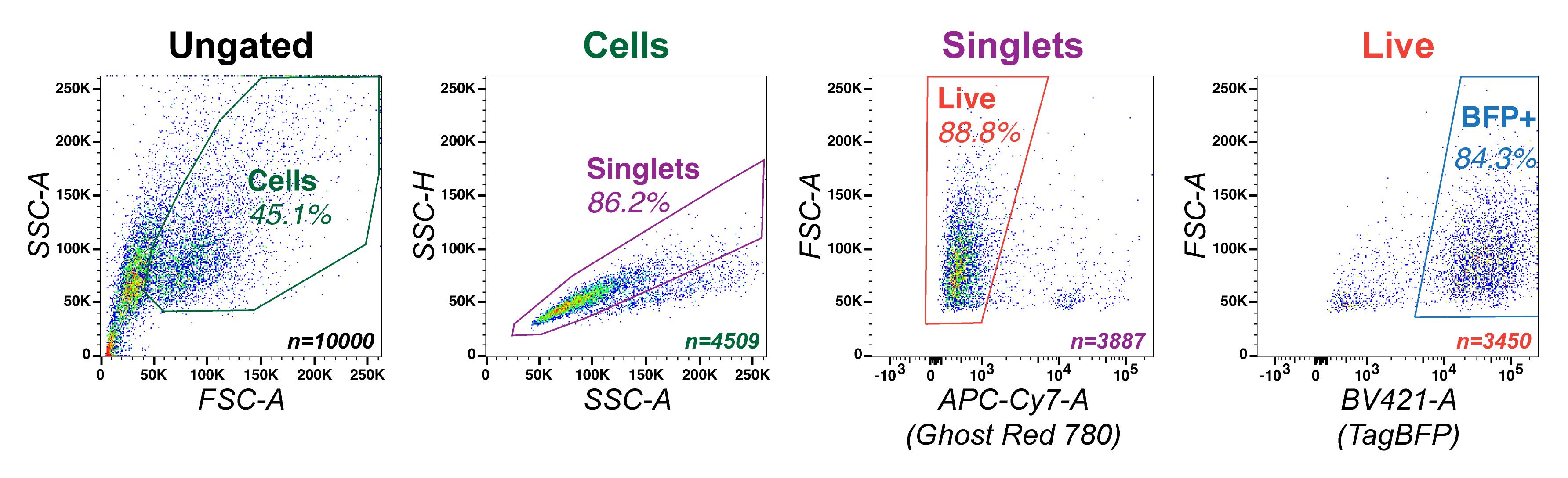
         Figure 5. Gating Strategy for Flow Cytometry. Representative example of a population of sgRNA-expressing dCas9-BFP-KRAB HepG2s, with sequential gates for cells (SSC-A vs. FSC-A, gate in green), single cells (SSC-H vs. SSC-A, gate in purple), live cells (FSC-A vs. Ghost Red 780, gate in orange), and BFP+ cells (FSC-A vs. TagBFP, gate in blue).

         
         

      3. Adjust the gains and voltages for the experiment, to achieve proper gating

         i. Open the instrument settings panel to adjust voltages for the appropriate channels.

         Note: Voltages adjust the sensitivity of the detectors on the instrument, with higher values increasing the values of the events on the axes of the plot. Discuss with the scientist maintaining the flow cytometer for beginning voltages for the cell type of interest, as these typically depend on cell size. Generally, aim to adjust voltages so that negative events range between 10¹ and 10² in arbitrary units, and the positive events are clearly identifiable, yet remain within the instrument’s limits of detection.

         ii. Transfer one well each of unstained parental cells and fully stained control cells to the 96-well plate used by the flow cytometer.

         Note: Resuspend cells by pipetting up and down prior to running samples, to prevent settling of cells. If no 96-well plate module is available on the flow cytometer, transfer cells to 1.2 mL “bullet” tubes that can fit inside a typical 5-mL FACS tube (the larger 5-mL FACS tube can be reused for each sample).

         iii. Begin running the unstained sample at low speed, and monitor readouts in real time, but do not record the data.

         Note: Stop the flow of cells once the voltages are established, as otherwise the machine will continue to aspirate cells and the sample will be fully consumed before the data are recorded.

         iv. Adjust FSC and SSC voltages to bring most of the cells into the gated region. Adjust gates as needed in real-time.

         Note: Debris should end up in the lower left corner of the FSC-A vs SSC-A plot, outside of the cell gate.

         v. Adjust the active fluorescent channel voltages other than TagBFP, to bring the values for the unstained cells to between 10¹ and 10².

         vi. Adjust the TagBFP fluorescent channel voltage, to bring the value for the unstained parental cells to between 10² and 10³.

         Note: The parental cells contain the dCas9-TagBFP-KRAB fusion, and will be positive for TagBFP. However, the brightness of cells harboring the free TagBFP protein from the CRISPRi/a vector is significantly higher than that of the parental cells with the TagBFP fusion. This allows differentiation of transduced from non-transduced cells .

         vii. Run the fully stained control sample at low speed, and monitor readouts in real time, but do not record the data.

         viii. Confirm that the FSC and SSC voltages are appropriate for the fully stained sample.

         ix. Adjust the active fluorescent channel voltages, to achieve a distribution of values that enables a clear distinction of the signal, yet remain within the dynamic range of detection for the instrument.

         Note: For the live-dead stain, the most positively fluorescent cells are nonviable, and will be excluded from analysis.

         x. Save the experimental template on the software, as well as the voltages for the instrument, so that both can be easily reloaded for future experiments.

      4. Run and collect the data on both control and experimental samples:

         i. On the software, create and label wells (or “tubes”) for each control and experimental sample.

         ii. Set the amount of volume to aspirate from each well and speed with which to run samples.

         Note: Expect to leave about 10 µL of sample in each well to avoid aspirating air into the fluidics lines. Samples will run faster if more concentrated and reconstituted in lower volumes. While samples will also run faster if run at higher speed, the accuracy of readouts may be reduced. This should be confirmed empirically, for the samples and the particular machine used.

         iii. Set the number of events to record. Typically, this is 1 × 10⁵ total events, but this number can be reduced, if necessary (e.g., if too few cells are available to record), or if a total number of “gated” events (i.e., cells) are desired.

         iv. Highlight and select the wells with the unstained cells, parental cells, and fully stained controls. Run these samples using an auto-record feature, if available on the machine.

         Note: Comparing the results of a fully stained control at the beginning of the experiment to one at the end will assess for any drift in the fluorescence channels.

         v. Using a multichannel pipette, transfer one row of cells (12 wells) to the 96-well plate to be used in the flow cytometer.

         Note: For live cells, transferring one row at a time allows cells to remain on ice longer until ready for analysis. This is not necessary for fixed cells or if the 96-well plate module for the flow cytometer is temperature controlled. Including a non-targeting control well at the end of each row permits a direct comparison between controls and experimental sgRNAs analyzed at similar timepoints after harvest and labeling.

         vi. Highlight and select the wells to run. Use the auto-record feature to run and record the samples.

         vii. Run and record a final fully stained control well at the end of the experiment.

      5. After all samples are run, clean and decontaminate the instrument:

         i. Export the raw data for each well as a .fcs file for data analysis.

         Note: Data analysis can also be performed on the machine’s software if desired.

         ii. Run the cleaning protocol for the instrument:

         1). For 96-well plates, this typically involves 3–5 wells of 10% bleach, followed by 5 wells of water.

         2). For individual tubes, this typically involves 3–5 min with a tube of 10% bleach at high speed, followed by 5 min of water at high speed.

         iii. Shut the machine down, according to the shut-down protocol.

Data analysis

1. Import raw flow cytometry data into the FlowJo analysis software, creating groups for experimental samples, biological controls, and non-targeting controls.

2. Concatenate data from all non-targeting control well files from a given plate into a separate file. Import this file into the group of non-targeting controls.

   Note: This step creates a control sample containing all events from the non-targeting control wells over the entire plate. This can improve sensitivity to detect a phenotypic effect of an experimental sgRNA, provided there is no significant fluorophore drift over the course of the experiment. Otherwise, the concatenated file may obscure a true effect.

3. Optional : Derive new parameters as desired for the experiment. Examples include ratiometric levels of fluorescence (e.g. Alexa-648^LDLR/Alexa-488^TFR), and fluorescence levels corrected for cell size (e.g. Alexa-648^LDLR/FSC-A). These derived parameters allow for ratiometric readouts at the single cell level.

4. Open the file from the first analyzed non-targeting sgRNA control, to draw gates and perform the template analysis:

   1. Gate for cells (FSC-A vs SSC-A), singlets (FSC-H vs FSC-A), live cells (FSC-A vs Ghost Red 780), and transduction (FSC-A vs TagBFP), and adjust axes as in F.b.ii. (see Figure 5).

      Note: Gating for live-dead cells or transduced cells can also be performed on histograms of the Ghost Red 780 or TagBFP channels, respectively. Such gating is simpler to apply, but does not account for differences in channel output correlated with cell size.

   2. On the fully gated population, open histograms of experimental fluorophore channels and derived parameters, to visualize the spread of data.

   3. Apply the desired statistics (i.e., total count, mean, median, and standard deviation) for the desired fluorophore channels and derived parameters, for the fully gated population.

5. Assess for experimental drift by comparing the first non-targeting sgRNA control well to the last non-targeting sgRNA control well of the experiment.

   Note: Differences between these samples can occur due to instrumental drift or to fluorophores fading over time. Both can be minimized by using either row-matched controls, or well-matched non-transduced controls.

   1. Apply the same gates and statistics to both wells.

   2. Overlay the data from both wells on the box plots and histograms, to visualize and qualitatively assess any differences.

   3. Quantify the difference in fluorophore channels:

      i. With the fully gated population (transduced, live, singlet cells) of the first control selected, open the “Compare Populations” tool in FlowJo.

      ii. Drag the same gated population of the last non-targeting sgRNA control into the “Compare Populations” window.

      iii. Select the desired parameter channels to compare, to obtain the Tχ metric.

      Note: The Tχ metric will provide a statistical likelihood that the populations are different, but does not imply there is a biological difference. The statistical test must be combined with the qualitative visualization of the histograms, as well as knowledge of the experimental details, to infer whether the biological effect is significant.

6. Determine the background fluorescence for each of the fluorophore channels.

   1. Apply the gates and statistics to the FMO negative control samples for each experimental parameter (i.e., Alexa-488, DiI, or Alexa-647). The mean and median of these values indicate the background fluorescence.

   2. If FMO controls are not available, the fully unstained control can be used. However, only the gates created with FSC and SSC parameters can be used to identify the desired cells.

7. Assess for whether additional compensation is needed due to fluorescence “spillover” between channels.

   1. Compare the experimental parameters in the FMO controls to the fully stained control. Apply the same gates and statistics to these controls, if not already done.

   2. Overlay the data from each fully gated FMO control to the fully stained control in the histograms of the experimental parameters, to qualitatively assess differences. A shift of the histogram in a particular channel in the fully stained control compared to the FMO control suggests spillover.

   3. Optional: If desired, the difference can be quantified by comparing populations, as in step 5.c.

   4. If spillover exists that affects the interpretation of the experiment, create a compensation matrix using the single-stained controls in the FlowJo software. This matrix can then be applied to the entire analysis.

8. Compare the experimental parameters in each of the experimental samples against control populations.

   1. Using non-targeting sgRNAs as controls:

      i. Apply the gates and statistics to the first experimental sample.

      ii. With the fully gated population of the first experimental sample selected, open the “Compare Populations” tool in FlowJo.

      iii. Drag the same gated population of the concatenated non-targeting sgRNA control into the “Compare Populations” window.

      iv. Select the desired parameter channels to compare, to obtain the Tχ metrics.

      v. Apply the gates, statistics, and comparison from the first experimental sample to the first experimental or biological control samples from each row of the plate analyzed.

      vi. For each of these samples, repeat the “Compare Populations” analysis with the non-targeting sgRNA control from the same row of the plate.

      vii. Apply all gates, statistics, and comparisons from the first experimental sample in each row of the plate analyzed to the remainder of the wells in that row.

      Note: The first comparison will be to the concatenated file and applicable to all experimental or biological control samples. The second comparison will be to the row-matched non-targeting sgRNA control.

   2. Using non-transduced cells from the same well as controls:

      Note: This comparison offers the advantage of comparing cells grown in the same well, but cannot be used if puromycin selection was performed.

      i. Select the population of live cells (Ghost Red 780 negative) in the first non-targeting sgRNA control sample.

      ii. Apply the desired statistics for the experimental parameters on both the TagBFP⁺ (transduced) and TagBFP^- (non-transduced) cells.

      iii. Perform the “Compare Populations” analysis of the TagBFP⁺cells to the TagBFP^- cells for this sample, as in 8.a.

      iv. Apply the same statistics and comparison to each experimental and control sample performed in the experiment.

9. Export the data in tabular format. Open the table window in FlowJo, and select the desired statistics and comparison metrics to export. Typically, this will include mean, median, standard deviation, total counts, and proportional counts for each population, as well as Tχ metrics for each comparison.

10. Optional : Create a graphical comparison of histograms for any biological controls or experimental samples desired [see Figures. S1B and C, S5A–C, S7A and B, S9A&B, S10A–D, and S11A–H in Smith et al. (2022) for examples]. Open the layout window in FlowJo, and drag the desired populations into the window to create the desired histograms. Given the number of samples analyzed in the experiment, a comparison of every sample is not interpretable on a single graph.

11. For comparison within a given experiment, evaluate the following for the individual sgRNAs:

    1. Use the total count of gated events to assess whether the data from a given well is interpretable.

       i. Total gated counts < 10% of the non-targeting control wells may be skewed and represent an inadequate sampling of the population, and should be interpreted with caution.

       ii. Low total gated counts but with normal proportion of live cells suggests a technical issue with the well. Consider censoring the data from these wells.

       iii. Low total gated counts with low proportion of live cells suggests toxicity of either the sgRNA or the gene knockdown.

    2. For interpretable wells, use the Tχ metric to assess the significance of the effect. The Tχ metrics of the biological controls can be used as a benchmark to correlate the statistical significance to the biological relevance of the effects.

12. Import the statistics (median, standard deviation, total counts) from the tabular data for each experimental parameter into data analysis software (e.g., Prism).

    Note: The median, rather than the mean, may better represent the data, given the skewed curves that typically exist in flow cytometry histograms.

13. Normalize the data for each sgRNA, using the background fluorescence as the minimum value and the result of the appropriate control (i.e., concatenated non-targeting sgRNA well, row-matched non-targeting sgRNA well, or well-matched non-transduced sample) as the maximum value. Repeat the normalization for each of these controls.

    Note: Normalization of the data allows for data to be combined and compared across experiments.

14. Compare the data by performing multiple t-tests against the selected control, adjusting the significance for multiple comparisons testing. The strength of effect (i.e., fold-change) and the adjusted p values of the biological controls can be used as a benchmark for the experimental sgRNAs.

15. To compare across multiple experiments, export the normalized tabular data into a spreadsheet.

    Note: Flow cytometry permits evaluation at the single cell level, and so each “event” can be considered a biological replicate. Nevertheless, consider performing at least three replicates of the experiment to ensure robustness of the findings.

16. Combine normalized data across multiple experiments by using the Cochrane method ( Higgins and Green, 2011), as follows:

    
    

    

    
    

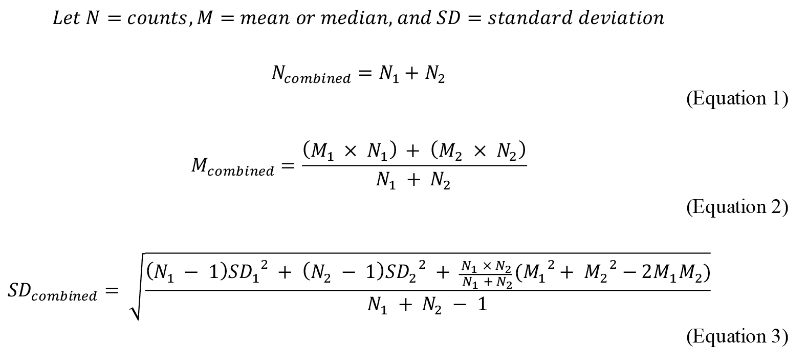
17. Iteratively combine data across replicate experiments.

18. As desired, import combined, normalized data into Prism, and repeat step 14.

    Data from individual or combined experiments can be log ₂ transformed in Prism, and then visualized in a heatmap (Figure 6).

    
    

    
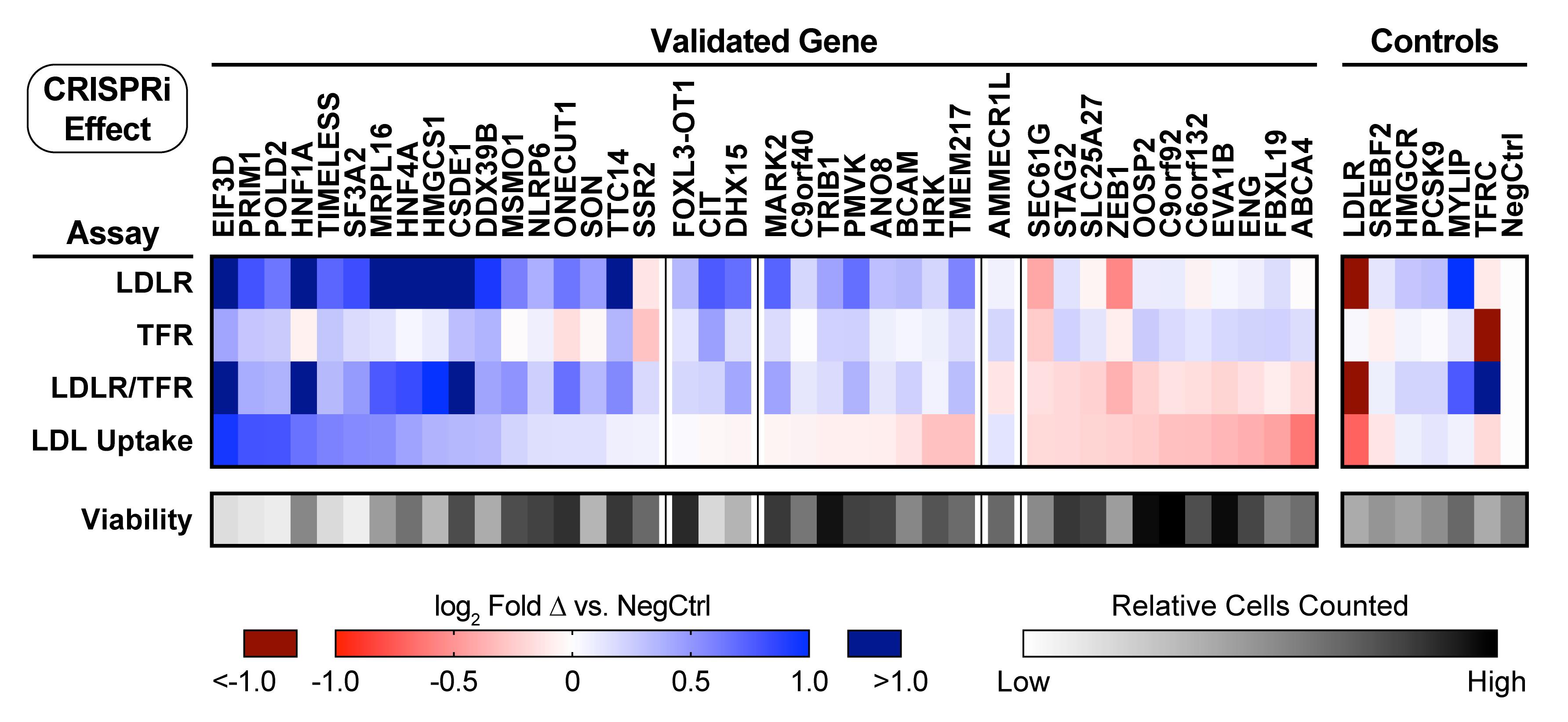
    Figure 6. Representative heatmap of sgRNA validation results. Heatmap showing receptor abundance (for LDLR, TFR, and the LDLR/TFR ratio) and fluorescent LDL uptake for dCas9-BFP-KRAB HepG2 cells transduced with sgRNAs targeting each indicated gene, as described in the above protocol. In this figure, hits are grouped first by the directional effect on LDLR abundance, and then by the effect on LDL uptake. Genes targeted as known controls are shown on the right. Readouts show the log₂ fold change compared to transduction with a negative control sgRNA, and represent the weighted average of the effects from two separate sgRNAs. Viability indicates the relative number of cells surviving to flow cytometry analysis in the experiments. All genes displayed had both sgRNAs independently validate for LDLR abundance, defined as p < 0.05 in the Holm-Sidak corrected t-test. Data represent summary information from four independent experiments. Figure modified from Smith et al. (2022).

Notes

1. Several online resources are available to assess for spectral overlap of fluorophores and design flow cytometry experiments, including FPbase (https://www.fpbase.org) (Lambert, 2019), and ThermoFisher Scientific’s Fluorescence SpectraViewer (https://www.thermofisher.com/order/fluorescence-spectraviewer).

2. Flow cytometry analysis software, such as FlowJo, can be used to automate compensation for overlapping fluorophores, if needed.

Recipes

1. 2× Annealing Buffer

   200 mM potassium acetate

   60 mM HEPES-KOH pH 7.4

   4 mM magnesium acetate

   To obtain proper pH, first make a 1 M stock solution of HEPES, and adjust to pH 7.4 with KOH, followed by sterile filtration. Then, combine the three reagents with an appropriate amount of Milli-Q H₂O, to make the 2× annealing buffer. Store at RT.

   
   

2. 50× TAE Buffer

   50 mM EDTA

   2 M Tris

   1 M acetic acid

   Combine solid Tris base with solid EDTA disodium, and dissolve completely in ¾ of the total volume of Milli-Q H₂O. EDTA will dissolve only at a mildly alkaline pH, thus the order of addition of the reagents is important. After dissolution, add glacial acetic acid, and bring to final volume with Milli-Q H₂O. The pH of the final buffer should approximate 8.6, and does not require adjustment. Store at RT.

   
   

3. 293T growth medium

   Add 50 mL of FBS to 500 mL of high glucose DMEM (for 10% v/v). Store at 4°C.

   
   

4. Viral harvest medium

   Add 1.1 g of BSA for every 100 mL of growth medium, followed by 1/100 volume of 100× penicillin-streptomycin. Dissolve and sterile filter. Store at 4°C.

   
   

5. HepG2 growth medium

   Add 50 mL of sterile FBS to 500 mL of low glucose DMEM (for 10% v/v). Store at 4°C.

   
   

6. Sterol-depleted medium

   Add 25 mL of lipoprotein-deficient serum to 500 mL of low glucose DMEM (for 5% v/v) and sterile filter. Store at 4°C.

   
   

7. FACS buffer (FB)

   To sterile PBS, add 1/100 volume and 10 U/mL DNase I. Mix to dissolve, and sterile filter. Store at 4°C.

   
   

8. DiI-LDL labeling medium

   Add 0.5% w/v BSA to serum-free low glucose DMEM. Mix to dissolve, and sterile filter. Store at 4°C.

Acknowledgments

JSC receives funding support from the NIH/NHLBI (K08 HL124068, R03 HL145259, R01 HL146404, R01 HL159457), the NIH/NIGMS (R21 141609), a Pfizer ASPIRE Cardiovascular Award, the Harris Fund, and the Research Evaluation and Allocation Committee of the UCSF School of Medicine. AP receives funding support from the Tobacco-Related Disease Research Program (578649), the AP Giannini Foundation (P0527061), the NIH/NHLBI (K08 HL157700), the Michael Antonov Charitable Foundation Inc., and the Sarnoff Cardiovascular Research Foundation. This protocol was derived and validated from original research described in Smith et al. (2022). We thank Matvei Khoroshkin for feedback on protocol implementation, and Kevan Shokat and the members of the Shokat laboratory for helpful discussion.

Competing interests

JSC has received consulting fees from Gilde Healthcare and Eko, unrelated to the published work. The other authors have no disclosures.

Ethics

No human or animal subjects were used in this protocol.

References

1. Bock, C., Datlinger, P., Chardon, F., Coelho, M. A., Dong, M. B., Lawson, K. A., Lu, T., Maroc, L., Norman, T. M., Song, B., et al. (2022). High-content CRISPR screening. Nat Rev Methods Prim 2(1): 8.
2. Cui, L., Vigouroux, A., Rousset, F., Varet, H., Khanna, V. and Bikard, D. (2018). A CRISPRi screen in E. coli reveals sequence-specific toxicity of dCas9. Nat Commun 9(1): 1912.
3. Davis, M. and Jorgensen, E. (2022). ApE, A Plasmid Editor: A Freely Available DNA Manipulation and Visualization Program. Front Bioinform 2: 818619.
4. Gilbert, L. A., Horlbeck, M. A., Adamson, B., Villalta, J. E., Chen, Y., Whitehead, E. H., Guimaraes, C., Panning, B., Ploegh, H. L., Bassik, M. C., et al. (2014). Genome-Scale CRISPR-Mediated Control of Gene Repression and Activation. Cell 159(3): 647-661.
5. Higgins, J. P. T. and Green, S. (Eds.). (2011). Cochrane Handbook for Systematic Reviews of Interventions Version 5.1.0. Cochrane, 2011. Available from www.training.cochrane.org/handbook
6. Horlbeck, M. A., Gilbert, L. A., Villalta, J. E., Adamson, B., Pak, R. A., Chen, Y., Fields, A. P., Park, C. Y., Corn, J. E., Kampmann, M., et al. (2016). Compact and highly active next-generation libraries for CRISPR-mediated gene repression and activation. Elife 5: e19760.
7. Horton, J. D., Goldstein, J. L. and Brown, M. S. (2002). SREBPs: activators of the complete program of cholesterol and fatty acid synthesis in the liver. J Clin Invest 109(9): 1125-1131.
8. Lambert, T. J. (2019). FPbase: a community-editable fluorescent protein database. Nat Methods 16(4): 277-278.
9. Loregger, A., Nelson, J. K. and Zelcer, N. (2017). Assaying Low-Density-Lipoprotein (LDL) Uptake into Cells. Methods Mol Biol 1583: 53-63.
10. Mandegar, M. A., Huebsch, N., Frolov, E. B., Shin, E., Truong, A., Olvera, M. P., Chan, A. H., Miyaoka, Y., Holmes, K., Spencer, C. I., et al. (2016). CRISPR Interference Efficiently Induces Specific and Reversible Gene Silencing in Human iPSCs. Cell Stem Cell 18(4): 541-553.
11. Qi, L. S., Larson, M. H., Gilbert, L. A., Doudna, J. A., Weissman, J. S., Arkin, A. P. and Lim, W. A. (2013). Repurposing CRISPR as an RNA-guided platform for sequence-specific control of gene expression. Cell 152(5): 1173-1183.
12. Reis, A. C., Halper, S. M., Vezeau, G. E., Cetnar, D. P., Hossain, A., Clauer, P. R. and Salis, H. M. (2019). Simultaneous repression of multiple bacterial genes using nonrepetitive extra-long sgRNA arrays. Nat Biotechnol 37(11): 1294-1301.
13. Shalem, O., Sanjana, N. E. and Zhang, F. (2015). High-throughput functional genomics using CRISPR-Cas9. Nat Rev Genet 16(5): 299-311.
14. Smith, G. A., Padmanabhan, A., Lau, B. H., Pampana, A., Li, L., Lee, C. Y., Pelonero, A., Nishino, T., et al. (2022). Cold shock domain-containing protein E1 is a posttranscriptional regulator of the LDL receptor. Sci Transl Med 14(662): eabj8670.