- Protocols

- Articles and Issues
- For Authors
- About
- Become a Reviewer

Targeting Ultrastructural Events at the Graft Interface of Arabidopsis thaliana by A Correlative Light Electron Microscopy Approach
Published: Vol 13, Iss 2, Jan 20, 2023 DOI: 10.21769/BioProtoc.4590 Views: 2973
Reviewed by: Wenrong HeYao XiaoAnonymous reviewer(s)
Original research article
The authors used this protocol in:
Jan 2022

Protocol Collections
Comprehensive collections of detailed, peer-reviewed protocols focusing on specific topics


Related protocols
Abstract
Combining two different plants together through grafting is one of the oldest horticultural techniques. In order to survive, both partners must communicate via the formation of de novo connections between the scion and the rootstock. Despite the importance of grafting, the ultrastructural processes occurring at the graft interface remain elusive due to the difficulty of locating the exact interface at the ultrastructural level. To date, only studies with interfamily grafts showing enough ultrastructural differences were able to reliably localize the grafting interface at the ultrastructural level under electron microscopy. Thanks to the implementation of correlative light electron microscopy (CLEM) approaches where the grafted partners were tagged with fluorescent proteins of different colors, the graft interface was successfully and reliably targeted. Here, we describe a protocol for CLEM for the model plant Arabidopsis thaliana, which unambiguously targets the graft interface at the ultrastructural level. Moreover, this protocol is compatible with immunolocalization and electron tomography acquisition to achieve a three-dimensional view of the ultrastructural events of interest in plant tissues.
Graphical abstract

Background
Plant grafting is a process that has been used for centuries in agronomy to combine interesting agronomical traits together, such as resistance and fruit productivity (Mudge, 2009), or to study systemic biological processes, such as epigenetic regulations and long-distance signaling (Molnar et al., 2010; Turnbull, 2010; Turnbull et al., 2002; Wu et al., 2013; Bidadi et al., 2014; Zhang et al., 2014; Yang et al., 2015). Despite its widespread use, the cytologic events required for the establishment of the graft union remain poorly understood (Gautier and Chambaud et al., 2019). During graft union formation, tissues from both partners have to undergo a process of dedifferentiation to form callus cells and set up new pathways of communication such as phloem, xylem, and plasmodesmata. The movement of dyes or fluorescent probes between the scion and the rootstock have been used to resolve the kinetics of vascular connection at the graft interface, but no ultrastructural data are available for the establishment of cell-to-cell connection via plasmodesmata (Melnyk et al., 2015; Melnyk et al., 2018). Knowledge of the ultrastructural mechanisms underpinning graft union formation is currently very limited because locating precisely the site of contact between the two grafted partners under electron microscopy is challenging due to the difficulty to distinguish the origin/identity of each cell at the graft interface, i.e. to distinguish between cells from the scion and cells from the rootstock (Kollmann et al., 1985; Kollmann and Glockmann, 1985, 1991; Pina et al., 2017; Notaguchi et al., 2020). Attempts were successfully made by Kollmann and Glockmann (1985) and Notaguchi (2020), in which plants from different species showing noticeable ultrastructural differences in the callus cells produced at the graft interface were used.
To overcome the requirement of cytological differences to accurately identify cell origin and properly localize the graft interface, we propose a protocol for correlative light and electron microscopy (CLEM) to unambiguously target the graft interface at the ultrastructural level. At present, the use of CLEM approaches is still scarce for the analyses of plant tissues (Bell et al., 2013; Marion et al., 2017). Two out of the three CLEM protocols developed for plants are unfortunately not easily compatible with electron tomography due to either the weakness of the embedded resin used (glycol methacrylate) or the absence of resin (Tokuyasu method) (Marion et al., 2017). The protocol described by Bell et al. (2013) presents the advantage of being easily accessible but, because it is based on a chemical fixation, only permits a coarse ultrastructural preservation. Here, in order to combine fluorescence and high ultrastructural resolution in the same sample, we adapted the protocol described by Kukulski et al. (2012a and 2012b), an in-resin fluorescence CLEM method for plant tissues (Kukulski et al., 2012a and 2012b). This protocol allows us to preserve fluorescence and maintain the ultrastructure; further, in combination with electron tomography, this method allows to reach a level of resolution enabling the visualization of the bilayer of the plasma membrane. Moreover, this protocol is compatible with immunogold labeling and is adapted for hypocotyls and roots of plantlets of Arabidopsis thaliana. For our study, the hypocotyl of a scion and a rootstock expressing a yellow fluorescent protein (YFP) and monomeric red fluorescent protein (mRFP), respectively, fused to the endoplasmic reticulum–retention motif HDEL, were grafted (Chambaud et al., 2022). By optimizing (1) the grafting procedure, (2) the duration of the freeze-substitution (FS) steps, (3) the thickness of the ultrathin sections, (4) the sample mounting for light microscopy (LM) observation, and (5) the LM acquisition, we were able to observe fluorescence signals and precisely target the graft interface. The compatibility of our CLEM protocol with our previously described electron tomography protocol (Nicolas et al., 2018), allowed to access the three-dimensional (3D) view of ultrastructural elements specifically at the graft interface (Chambaud et al., 2022). Our CLEM protocol has the potential to unravel multiple plant cell processes at the ultrastructural level and was in fact already applied successfully to study autophagy (Gomez et al., 2022) and phase-to-phase separation processes (Dragwidge et al., 2022).
Materials and Reagents
Plant culture
1.5 mL Eppendorf tubes (Sarstedt, catalog number: 72.708)
12 N or 37% hydrochloric acid (Carlo Erba, catalog number: 524526)
1.5 mL Eppendorf tube rack (Ratiolab cardboard grid, inserts for cryobox, catalog number: 5020147)
Square plastic culture plates for A. thaliana seedlings, vertical culture (VWR, catalog number: 391-0444)
Bleach (Orapi Europe, catalog number: OR0011)
Murashige and Skoog (MS) medium + vitamins (Duchefa Biochemie, catalog number: M0222.0050) for seedlings
Plant agar for seedlings culture and grafting (Duchefa Biochemie, catalog number: P1001.1000)
Anapore tape (Euromedis, catalog number: 135320) to seal culture plates
KOH
Bleach solution for seeds sterilization (Recipe 1)
Culture medium for seedling and grafting (Recipe 2)
Half-strength MS medium for seedlings
Water medium for grafting
Transgenic lines
For grafting experiments, we used 35S::HDEL_mRFP and 35S::HDEL_YFP lines, which have strong fluorescent expression (Nelson et al., 2007;Lee et al., 2013). Both lines showed a fluorescence signal that was easily visible through oculars with a zoom microscope with the medium pre-set level for the excitation power and the adapted set filter.
Plant grafting
Round Petri dishes, 90 × 14.2 mm for grafting (generally used for bacterial culture) (VWR, catalog number 391-0439)
Neutral nylon membrane hybond-N (GE Healthcare, catalog number: RPN 203 N)
Paraffin film (Bemis, Parafilm ‘M’) cut into strips of approximately 1 cm wide to seal the Petri dishes
High-pressure freezing (HPF)
Screw-top 2 mL tubes (Sarstedt, catalog number: 72.693)
Toothpicks
Bovine serum albumin (BSA) fraction V (Sigma-Aldrich, catalog number: 05482)
Methyl cyclohexane (MCH) (Merck Schuchardt OHG 85662 Hohenbrunn, Germany)
Distilled water to cut sample
Membrane carriers (100 μm deep with 1.5 mm diameter) (Leica Microsystems, catalog numbers: 16707898)
20% BSA solution for cryoprotection during HPF (see Recipe 3)
Freeze-substitution (FS)
Disposable regular pipettes, 1, 2, and 3 mL (VWR, catalog numbers: 612-2850, 612-2851, and 612-1681) and FS-specific 1 mL pipettes with thin tips (Ratiolab, catalog number: 2600155)
Wheaton glass sample vials with snap-cap for cryomix preparation (DWK Life Sciences, WHEATON, catalog number: 225536)
Personal cartridge half mask 6100 (Honeywell International, catalog number: 1029471)
Aluminum foil
Uranyl acetate powder (Merck, catalog number: 8473)
Pure methanol (Fisher Scientific, catalog number: M/4062/17)
Ultrapure 100% ethanol and acetone (VWR, catalog numbers: 83813.440 and 20066.558, respectively)
Colored nail polish (color does not matter)
12.5 mL reagent containers with screw caps (Leica Microsystems, catalog number: 16707158)
HM20 resin (Electron Microscopy Sciences, catalog number 14345)
Reagent bath (Leica Microsystems, catalog number: 16707154)
Plastic mold flow-through rings (Leica Microsystems: 16707157)
Cryosubstitution uranyl-acetate stock solution (20%) (see Recipe 4)
Cryosubstitution mix (see Recipe 5)
HM20 solutions (see Recipe 6)
Ultramicrotomy
Crystallizing dish (Fisher Scientific, catalog number: 11766582)
Fast absorbent paper filters (Whatman, Filter papers 41) (GE Healthcare, catalog number: 1441-070)
Glass rods (Fisher Scientific, catalog number: 12441627)
Gilder standard hexagonal 200 mesh copper grids (Electron Microscopy Sciences, catalog number: G200HS-Cu) to coat with parlodion or commercial grids with formvar (Electron Microscopy Sciences, catalog number: FCFT200-CU)
Razor blades for coarse block preparation (Electron Microscopy Sciences, catalog number: 71990)
Pasteur pipet (VWR, catalog number: 612-1720)
0.2 μm syringe filter (VWR, catalog number: 514-0061)
10 mL syringe (Terumo, catalog number: SS+10ES1)
Solid parlodion (Electron Microscopy Sciences, catalog number: 19220)
Isoamyl-acetate (Sigma-Aldrich, catalog number: W205532)
Toluidine blue powder (Sigma-Aldrich, catalog number: T3260)
Sodium borate powder
Ultrapure (Milli-Q) water
2% parlodion solution for grid filming (see Recipe 7)
Toluidine blue solution (see Recipe 8) for screening block sections on tabletop microscope during resin block milling
Electron microscopy
Gold colloid 5 nm (BBI Solution, catalog number: EMGC5)
Gold fiducials solution (see Recipe 9)
Equipment
Plant culture
Desiccator used as hermetic chamber
Fume hood
Glass crystallizing dish
Fridge for vernalization
-80°C freezer for sterilization
Plant grafting
Dissecting microscope with a minimal working distance of 5 cm (Leica Microsystems, model: Leica MZFLIII)
Glass beaker for sterilization of tools with ethanol
Spray for ethanol
Dissecting micro-knives 15° 5 mm (Fine Science Tools, catalog number: 72-1551)
Precision tweezers [EMS style 5X, catalog number: 78320-5X (soft) and 78520-5X (hard)]
Fluorescence screening
Zoom microscope (Zeiss Axiozoom.V16) equipped with a 0.5× objective with a numerical aperture of 0.125. The fluorescent part is composed by the fluorescence source Optoprim sola SE II and filter sets (GFP filter set: excitation window between 460 and 480 nm and emission window between 500 and 548 nm; mRFP filter set: excitation window between 540 and 580 nm and emission window up to 593 nm).
High-pressure freezing (HPF)
Liquid nitrogen, liquid nitrogen container, and adapted personal protection gear
Air compressor (JUN-AIR)
Leica EM-PACT1 machine (Leica Microsystems)
Leica loading system
Pod holders (Leica, catalog number: 16706832)
Pods (Leica, catalog number: 16706838)
Regular biomolecular pipettes, ranging from 2 to 1,000 µL
Binocular with transmission illumination for root dissection (Nikon, model: SMZ-10A)
Heating surface for quick drying of pods and pod holders during the session
Insulated tweezers for manipulation in liquid nitrogen (VOMM Germany, 22 SA ESD)
Metal containers for frozen sample transfer and associated screwdriver for lifting procedures (provided with EMPACT1)
Torque screwdriver (TOHNICHI, Torque driver RTD60CN) set to 30 N.cm
Freeze-substitution (FS)
Leica automatic freeze-substitution AFS2 (Leica Microsystems, model: Leica AFS2)
Leica freeze-substitution processor FSP (Leica Microsystems, model: Leica FSP)
Metal socket for mold containers
Microneedles for separating the membrane carriers from frozen samples [microneedle 0.025 mm (Electron Microscopy Science, catalog number: 62091-01) and 5 µm (Ted Pella, catalog number: 13625)]
Ventilated fume hood
Ultramicrotomy
Block holders
Diamond trimming knife for first milling steps to reach the sample (Drukker 8 mm Histoknife Dry, discontinued)
Diamond knives Trim20 dry (Diatome, catalog number: DTB20), Ultra wet 45° (Diatome, catalog number: DU4530), and Histo wet (Diatome, catalog number: DH4560)
ELMO glow discharger (optional) (CORDOUAN Technologies)
Grid carriers for grid storage
Leica Ultracut UC7 (Leica Microsystems, model: Leica Ultracut UC7)
Tabletop microscope (Olympus, model: CX-41)
Precision weight scale for parlodion weighting (Sartorius, model: TE124S)
Confocal microscopy
Sensitive confocal microscope (Zeiss Microscopy, model: Zeiss LSM 880) and 63× NA 1.4 oil immersion objective
Electron microscopy
FEI Tecnai G2 Spirit 120 kV equipped with Eagle 4K × 4K high sensibility CCD camera
Advanced tomography holder (Fischione instruments, model: 2020)
Software
Zeiss Zen Dark version 2.3 software (https://www.zeiss.com/microscopy/int/products/microscope-software/zen.html) used for confocal acquisition
Tecnai imaging and analysis (TIA) version 4.5 software was used in conjunction with transmission electron microscopy (TEM) User Interface software version 4.5 to control and acquire micrograph with the electron microscopy (https://www.fei.com/software/)
Xplore3D version 4.5 (FEI) was used for automated tilt series acquisitions (https://www.fei.com/software/)
ImageJ version 1.53n (https://imagej.nih.gov/ij/download.html) with the Bio-Format version 6.9 plugin (https://www.openmicroscopy.org/bio-formats/) to open and process the Zeiss .czi files and to open the .mrc tilt series files and tomograms.
IMOD suite version 4.11.6 (http://bio3d.colorado.edu/imod/). All processing of tomograms was done using the IMOD suite (Kremer et al., 1996), from the alignment of the tilt series to tomogram reconstruction
For visualization purposes only, Adobe Photoshop version 23.0.1 is used for TEM mosaic assembling using photomerge function.
ICY version 2.4.2.0 and its plugin ec-CLEM version 1.0.1.5 (https://icy.bioimageanalysis.org/plugin/ec-clem/) were used for LM and TEM correlation
Procedure
Plant grafting
The A. thaliana hypocotyl grafting procedure was adapted and optimized from the Two Segment Shoot-Root Graft part of the protocol of Melnyk (2017a) . Finding the good level of humidity is the most challenging part of Melnyk’s protocol. In our hands, replacing the water-soaked Whatman paper by a water-based agar medium was key to maintain constant humidity for several days after grafting and increased our grafting success from 50% to 80%. To target the graft interface with CLEM, we grafted transgenic lines expressing fluorescent proteins fused to the endoplasmic reticulum–retention motif HDEL (35S::HDEL-YFP and 35S::HDEL-mRFP1.2) ( Dean and Pelham, 1990 ; Knox et al., 2015; Chambaud et al., 2022). The constitutive 35S promotor was used to ensure a strong initial fluorescent signal.
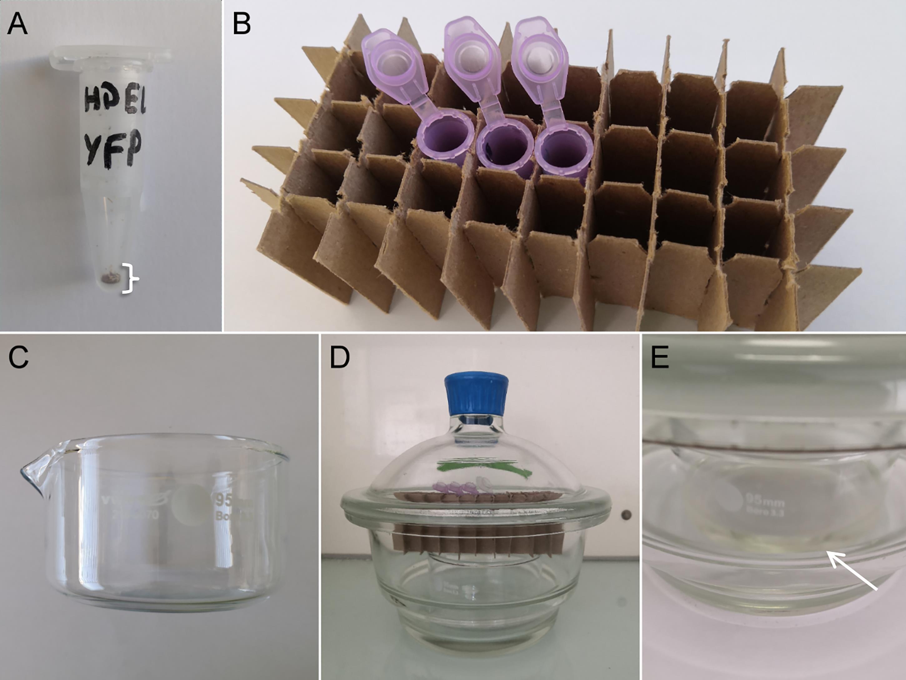
Figure 1. Seed sterilization procedure. (A) Appropriate number of seeds in a 1.5 mL sample tube for a proper sterilization. (B) For gas sterilization, place them open in a tube rack. (C) Glass crystallizing dish for the bleach. (D) Hermetic chamber with bleach in the glass crystallizing dish, tube rack, and open Eppendorf tube containing seeds. (E) When mixing bleach with hydrochloric acid, the solution becomes yellow (white arrow) and a faint yellow haze of chloride gas is visible.Plant culture
Sterilize A. thaliana seeds with chlorine gas (adapted from Lindsey et al., 2017).
Aliquot a small number of seeds (approximately 100–150) into a 1.5 mL centrifuge tube labeled with a permanent pen (covered in adhesive tape to avoid washing off of the ink), close the caps, and place them for 20 min in a -80°C freezer (Figure 1A).
The sterilization will take place in a hermetic chamber, typically a glass desiccator, under a fume hood. In the desiccator, place a small glass crystallizing dish containing 50 mL of bleach solution (see Recipe 1) (Figure 1C and 1D).
Uncap centrifuge tubes before placing them in a tube rack in the chamber. Add 1.5 mL of 12 N hydrochloric acid to the bleach solution that is in the crystallizing dish without mixing and quickly close the chamber. The yellow haze of chlorine gas should be visible at this point (Figure 1E). Let the seeds in the chamber from 4 h to overnight (e.g., 6 pm–9 am).
Open the chamber and close the centrifuge tubes. Leave the chamber open under the fume hood for one day until the reaction between hydrochloric acid and bleach ends. The reaction produces chlorine gas, sodium chloride, and water. You can then discard the solution. Note that if the seed germination seems affected, the incubation time should be reduced to 1–3 h.
Under a laminar flow hood, gently sprinkle the seeds over square Petri dishes containing half-strength MS medium with vitamins. Thanks to chloride gas sterilization, homogeneous distribution of the dry seeds is easily achieved. Seal the plate with anapore tape.
For vernalization and stratification, place the plates horizontally with the seeds on the upper face at 4°C in the dark for 2–5 d maximum.
Transfer the plates to a growth chamber regulated at 20–23°C with photosynthetic photon flux density (PPFD) of 100 µmol·m-2·s-1 of light. Put the plates vertically so that the hypocotyls grow as straight as possible. Note that short-day growing conditions (such as 8 h of light per day) give rise to more elongated and thinner hypocotyls, which facilitate the grafting procedure and microscopy experiments (Melnyk, 2017a, 2017b). Once the two first true leaves are just visible under the binocular microscope, grafting can be done (Figure 2). In general, seedlings grown under short or long days (i.e., 8 and 16 h of light) have to be 5 or 7 days old, respectively, for grafting. At all times, you need to monitor plant growth to graft at the more appropriate time.
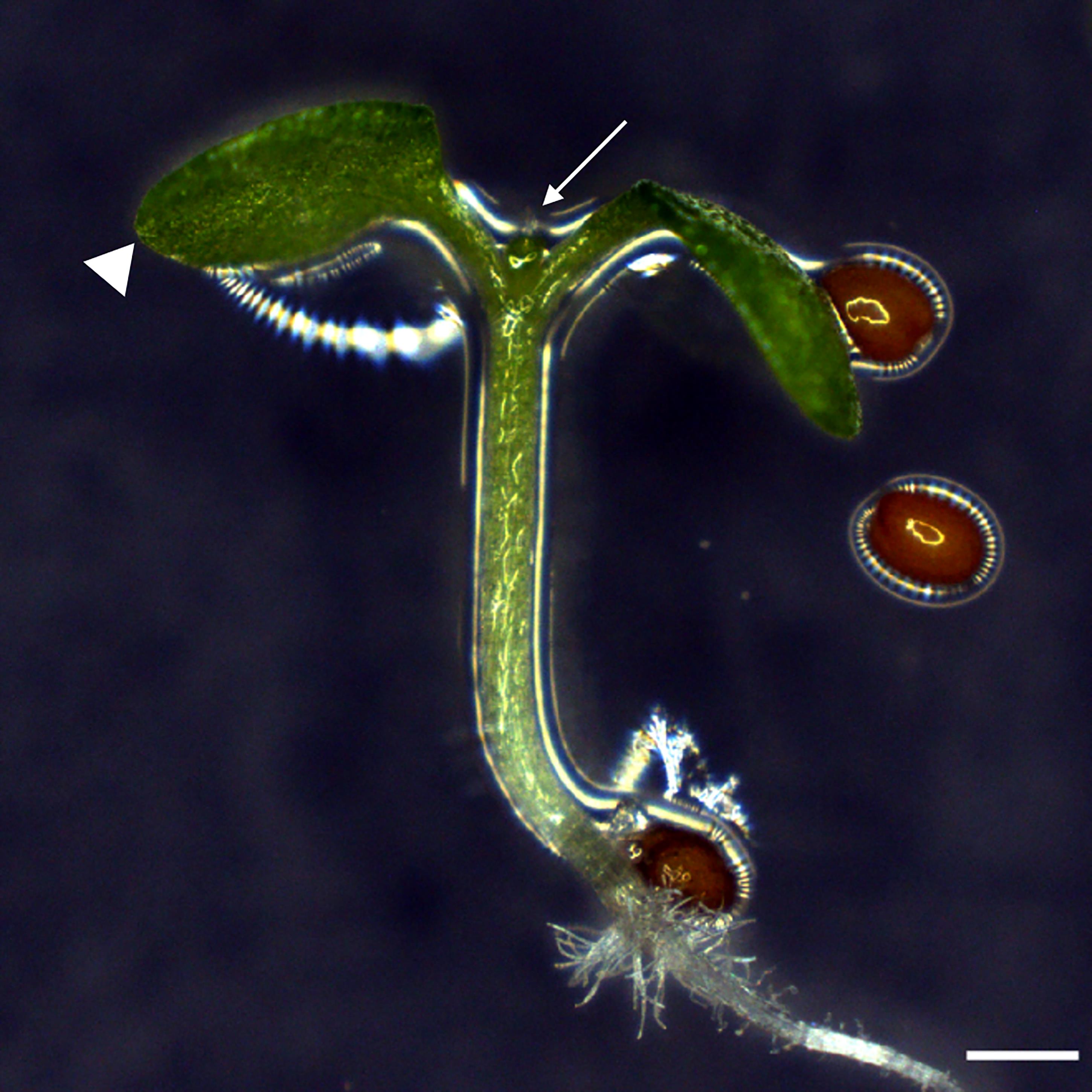
Figure 2. The ideal Arabidopsis plantlets for grafting. An idealA. thaliana seedling for grafting has a straight hypocotyl, very small first leaves (white arrow), and cotyledons that should not bend over the hypocotyl (white arrowheads). Scale bar: 500 µm.
Grafting
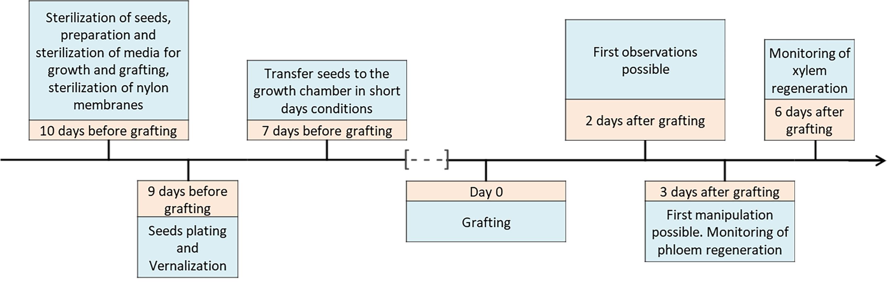
Figure 3. Workflow of grafting experimentsThe absence of sucrose in the culture and grafting media makes it possible to graft in non-sterile conditions if you do not plan to keep the grafts in vitro for more than six days. In our grafting studies, we grafted on the bench in non-sterile conditions because we worked on samples at three and six days after grafting. Nevertheless, we work on a 70% ethanol pre-cleaned bench with sterilized tools to limit contamination.
The dissecting microscope used must have a working distance (distance between the lens and its focal plane) of at least 5 cm to allow enough space for the manipulations. We usually use a magnification between 6× and 20× with annular illumination or optical fiber systems. Performing grafting is tedious and requires precise and quick manipulations. Try to avoid coffee and other stimulants before attempting grafting experiments. With practice, the grafting technique allows you to reach a success rate of 80% to 90% with a rate of 70 grafts per hour. Following the workflow of grafting experiments proposed (Figure 3) can help you to organize your schedule. For the grafting day, book the epifluorescence zoom microscope and the stereomicroscope and prepare the material (Figure 4).
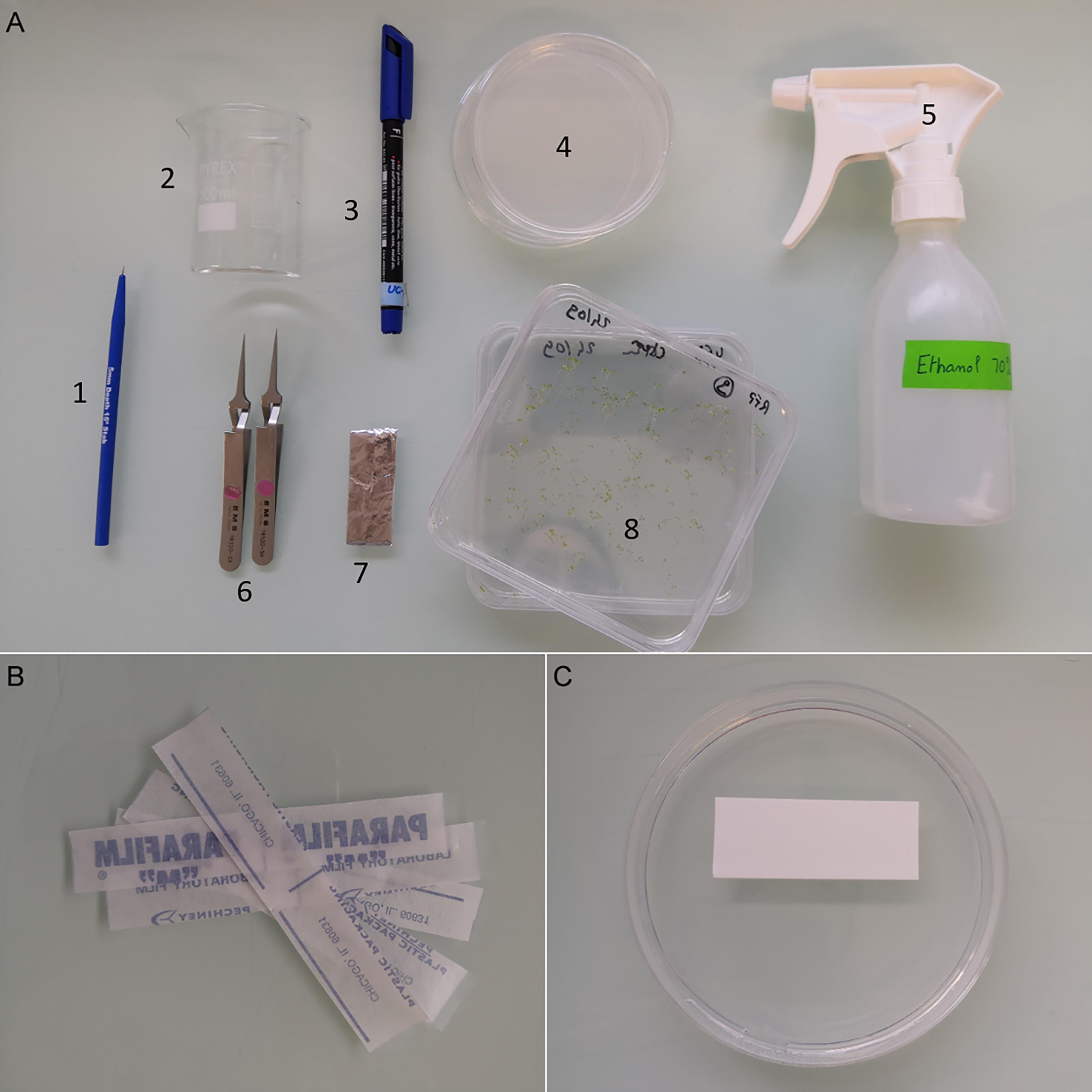
Figure 4. Grafting tools. (A) 1. Dissecting micro-knife for grafting; 2. Glass beaker for sterilization of tools; 3. Permanent marker to label Petri dishes; 4. Round Petri dishes for grafting; 5. Spray with ethanol for tools and bench cleaning; 6. Fine tweezers; 7. Sterile nylon membrane wrapped in aluminum foil; 8. Plants to graft. (B) Parafilm strips to seal Petri dishes after grafting. (C) Positioning of nylon membrane prior to grafting.Before grafting
Cut a nylon membrane in 2 × 5 cm pieces and wrap them in aluminum foil.
Prepare the grafting medium with 1.6% plant agar in distilled water and buffer it at pH 5.8 with 1 N KOH.
Autoclave the grafting medium and the pieces of nylon membranes wrapped in aluminum foil at 120°C for 20 min.
When the grafting medium is handleable (avoid burns after autoclaving), fill the round Petri dishes with approximately 20 mL of agar under a laminar flow hood.
For grafting step
Using a fluorescence zoom microscope with an excitation power set at the medium pre-set level, identify plantlets showing a strong expression of fluorescence with excitation power.
Gather Petri dishes, micro-knives, tweezers, nylon membranes, permanent pen, and strips of parafilm (Figure 4).
Clean the dissecting microscope, micro-knives, and tweezers by spraying 70% ethanol and let them dry completely before usage. If you have to graft more than two plates, repeat the cleaning step every two plates.
Label your Petri dishes with the plant lines you will use as the scion and the rootstock.
Put a piece of nylon membrane on the upper part of each box (Figure 4C).
Among fluorescent plantlets, select the ones with homogeneous size, hypocotyls as straight as possible, and cotyledons not bent over hypocotyls (Figure 2). Put them in a row on the membrane (Figure 5). To move them, you can use tweezers or a toothpick that does not pinch the tissue. Note that you have to avoid any damage to the hypocotyl, shoot, and root. If you want to use the two genotypes as scion or rootstock, you could put six plants of the first genotype in the same row of six plants of the second genotype (Figure 5A). If you wish to use a genotype only as scion and the other only as rootstock, you could dispose the plants in two rows of 12 plants (Figure 5B).
The membrane is used as a cutting surface. Cut on it to avoid damages to the micro-knife.
Notes:
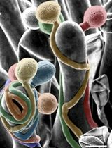
If the micro-knife is used properly, each can be used for approximately 400–500 grafts. It must permit a sharp sectioning in only one movement. Under a cleaned dissecting microscope, cut off and discard one cotyledon (choose the smallest, most damaged cotyledon that is bent over the hypocotyl) to allow the seedling to lie flat on the membrane (Figure 6A, B, C). Cut transversally through the hypocotyl, just under the cotyledons, without crushing the plant (Figure 6D).
Cutting the hypocotyl too low could impair the grafting success due to the formation of adventitious root from the scion (Video 1).
 Video 1. Arabidopsis thaliana hypocotyl grafting
Lift the scion by the petiole with closed tweezers and place it against the rootstock of another plant (Figure 6F and 6G). Most of the surfaces of both sectioned parts have to be in contact. You can improve the positioning by gently pushing the cut scion against the cut rootstock with the closed tweezers to bring both partners in direct contact (Figure 6G and 6H).
Note: We recommend that you graft together hypocotyls with similar diameters and avoid moving the cut rootstock, which is very fragile. The moisture level is crucial during graft union formation. Grafting onto grafting medium (water with 1.6% agar) keeps the moisture level constant and allows to keep the grafts in vitro six days after grafting.
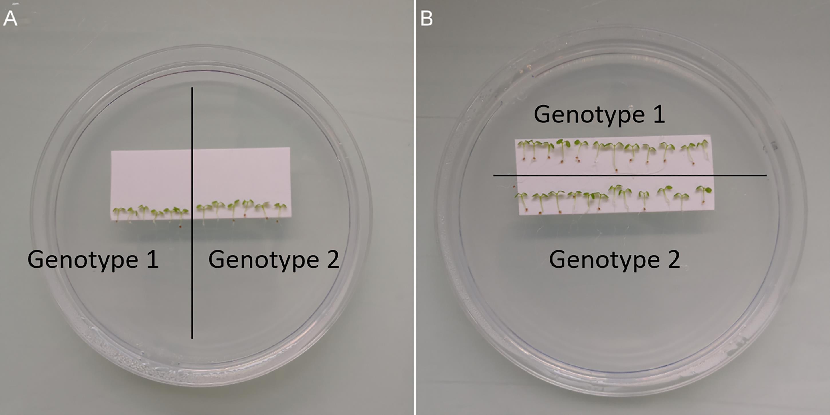
Figure 5. Grafting preparation. (A) When wishing to keep both directions of grafting (genotype 1/genotype 2 and genotype 2/genotype 1), a 6/6 graft scheme can be used. Scions and rootstocks will be prepared, cut, and exchanged between the two genotypes. (B) When a single direction of grafting is required (genotype 1/genotype 2 as above), a 12/12 graft scheme can be used. Bring the scions on the top row (genotype 1) before cutting and discarding their roots. The bottom row (genotype 2) contains rootstocks. Their apical part will be cut and discarded. Scions prepared from genotype 1 will be moved and grafted to rootstocks from genotype 2.Repeat steps c., d., and e. until all the plants are grafted. To save time, you can do this in a row: (1) cut and discard one cotyledon on each seedling, (2) cut all the shoots, (3) move them next to the prepared rootstocks, (4) align and push the scions onto the rootstocks.
When the grafting is done, be very cautious with the plates to avoid sudden movements that could induce the scion falling off the rootstock. Close the lid and seal the plates with a Parafilm strip. You can label the plate with the time you ended grafting so that you know the age of the graft. Carefully put the plate vertically back in the growth chamber at 20–23°C in PPFD of 100 µmol·m-2·s-1 light in either short- or long-day conditions. Note: If you grafted properly, you can begin to manipulate your graft (i.e., observing it under a microscope, fix tissues, transferring it to a new medium, etc.) 48 h after grafting. After 3 d, the grafts become slightly more robust as phloem should be connected. After 6–7 d, xylem is connected, and the grafted plant becomes quite robust. When beginning grafting experiments, you may need to assess your grafting success rate at first. You can rely on several criteria to evaluate grafting success (Melnyk, 2017b), such as the resumption of root growth, usually with emergence of lateral roots, and the absence of adventitious root formation in the scion. You can also monitor the phloem connection by grafting scions expressing pSUC2::GFP [i.e., green fluorescent protein (GFP) under the phloem-specific SUC2 promoter] and observing the movement of GFP to the rootstock, or by applying carboxyfluorescein diacetate (CFDA) to the scion or rootstock to evaluate phloem and xylem connectivity as described in Melnyk (2017b).
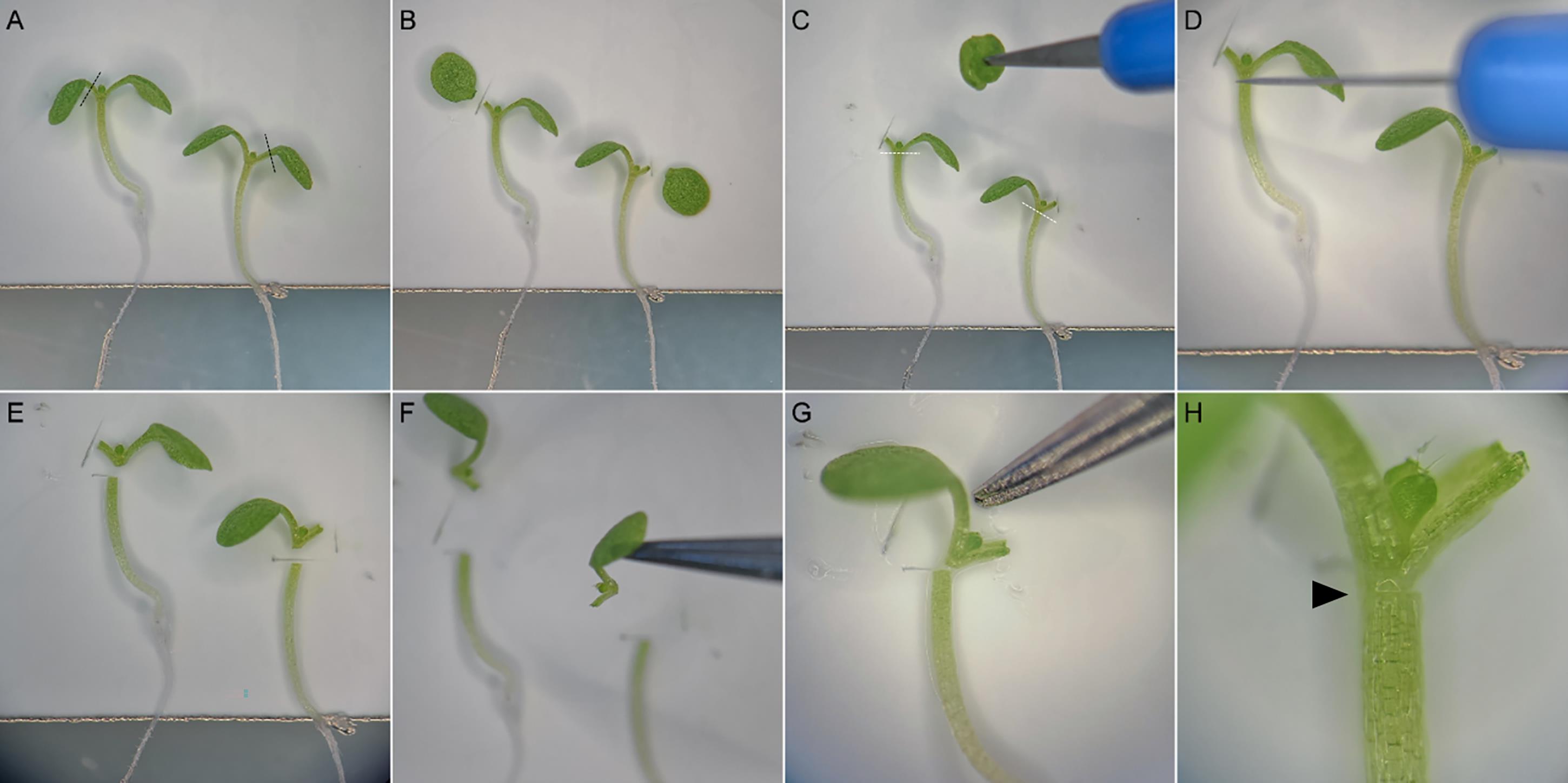
Figure 6. The step-by-step procedure of grafting. The two plants are placed side by side on a nylon membrane and one cotyledon of each plant is cut along the black dashed lines (A and B) and then discarded (C). Hypocotyls are cut just below the petiole of cotyledons along the white dashed lines (D and E). Scions are exchanged between plants by sticking them to the tip of the tweezers (F). Scion is carefully brought close to the rootstock with the tip of the tweezers (G). When properly grafted, the graft junction (black arrowhead) is barely visible (H).
CLEM
Before fixation, ensure that the fluorescence signals are easily visible through the oculars for individual samples with non-destructive observations (stereomicroscopy or macroscopy).
HPF
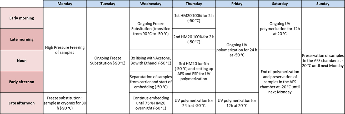
Note: HPF was done using the Leica EM-PACT1 machine (Studer et al., 2001). A detailed protocol is described in Nicolas et al. (2018). This procedure involves the manipulation of liquid nitrogen; if you are not familiar with its handling, please refer to the official guidelines. Moreover, we recommend fixing approximately 10 samples by condition and to process all your samples of one condition as a batch, before fixing the next one. It will help you avoid mixing up the different grafts. Moreover, we recommend starting the HPF and FS either on Monday or Tuesday to finish handling for block preparation on the next Thursday or Friday (Table 2).
Prepare the EM-PACT1 machine by (1) filling its dewar with liquid nitrogen, (2) filling the MCH chamber, and (3) evacuating the air out the circuit by two blank shoots.
Charge the membrane carrier (100 µm deep carriers) on the Leica loading system.
Pick a grafted plant out of the Petri dish and place it on a glass slide covered with water under a binocular zoom microscope.
Note: The following steps should be carried out as fast as possible to limit biological responses from the cutting and BSA drying.
Fill the carrier with 20% BSA in water with a 0.5–2 µL pipette until the liquid surface is domed in the well of the carrier. Ensure that there are no air bubbles.
Under the binocular zoom microscope, dissect the graft interface in water on a glass slide with a razor blade and then carefully pick it up with a toothpick.
Dispose the graft interface into the BSA in the membrane carrier before pushing the membrane carrier in the pod using the Leica loading system.
Close the pod using the Torque screwdriver (set on 30 N.cm) and remove the Leica loading system.
Load the sample in the EM-PACT1 machine and shoot.
Check the freezing rate and pressure rise on the screen by ensuring that maximum pressure is reached approximately 20 ms before reaching the minimal temperature.
Store your frozen sample under at least -90°C until the FS step.
Repeat steps B1b–j until all your samples are frozen.
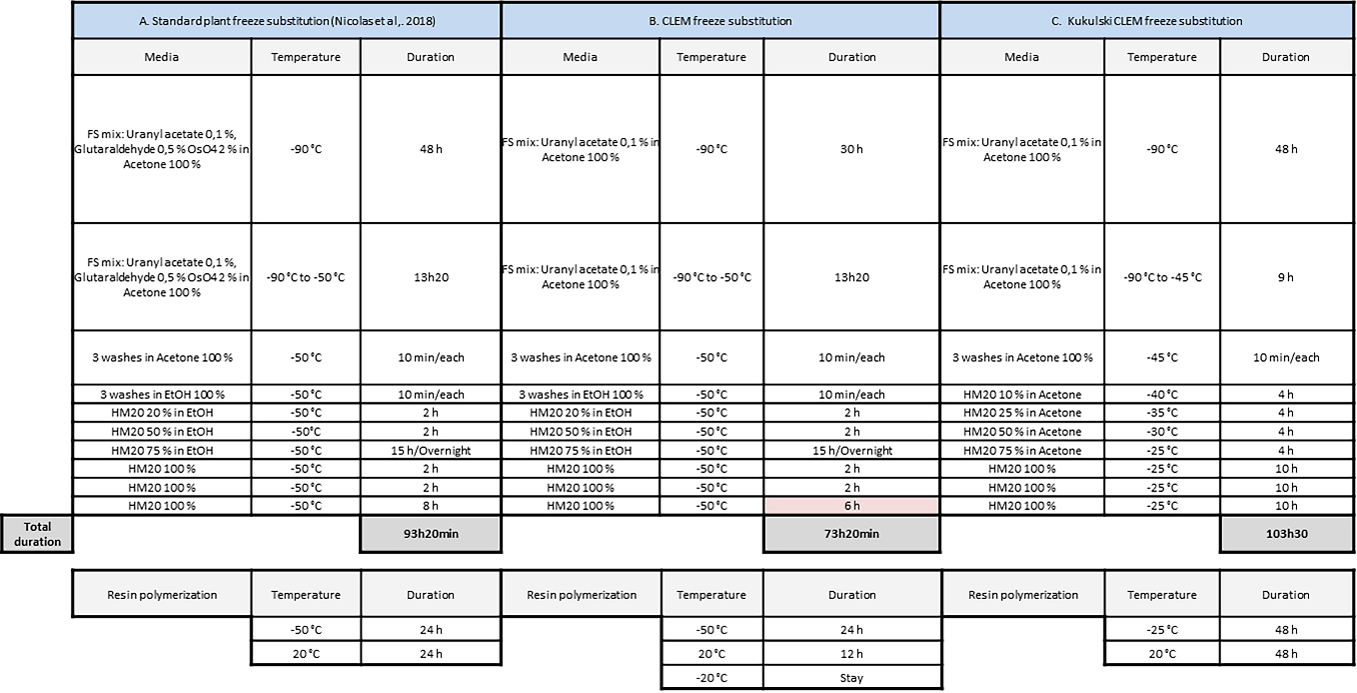
Table 1. Plant correlative light electron microscopy (CLEM): freeze substitution (FS) and resin polymerization program compared to standard plant and yeast CLEM programs
Freeze-substitution (FS)
Note: Our FS and embedding protocol is based on the protocol published by Kukulski et al. (2012a and 2012b); it was initially designed for yeast and mammalian cells and we adapted it for our plant tissues (Table 1). During the FS and until the dehydration of the samples, it is crucial to maintain the sample under -80°C to avoid the formation of ice crystals. For this purpose, every container, medium, and tool has to be precooled before entering in contact with the frozen samples. This procedure involves the manipulation of liquid nitrogen, uranyl acetate, and HM20. If you are not familiar with the handling of these compounds, please refer to the official guidelines. Uranyl acetate should be preserved from light to prevent the formation of precipitate. Nevertheless, there is no need to work in the dark; avoiding direct and long light exposition of solutions with uranyl acetate as much as possible is sufficient. We can process from one to four different conditions per FS experiments with five to ten samples per condition. To ease the manipulation, the samples of the very same condition are mixed together in the same FS reagent bath (Figure 7). Between each bath, do not remove all liquid, systematically letting a background of liquid to avoid drying of samples.
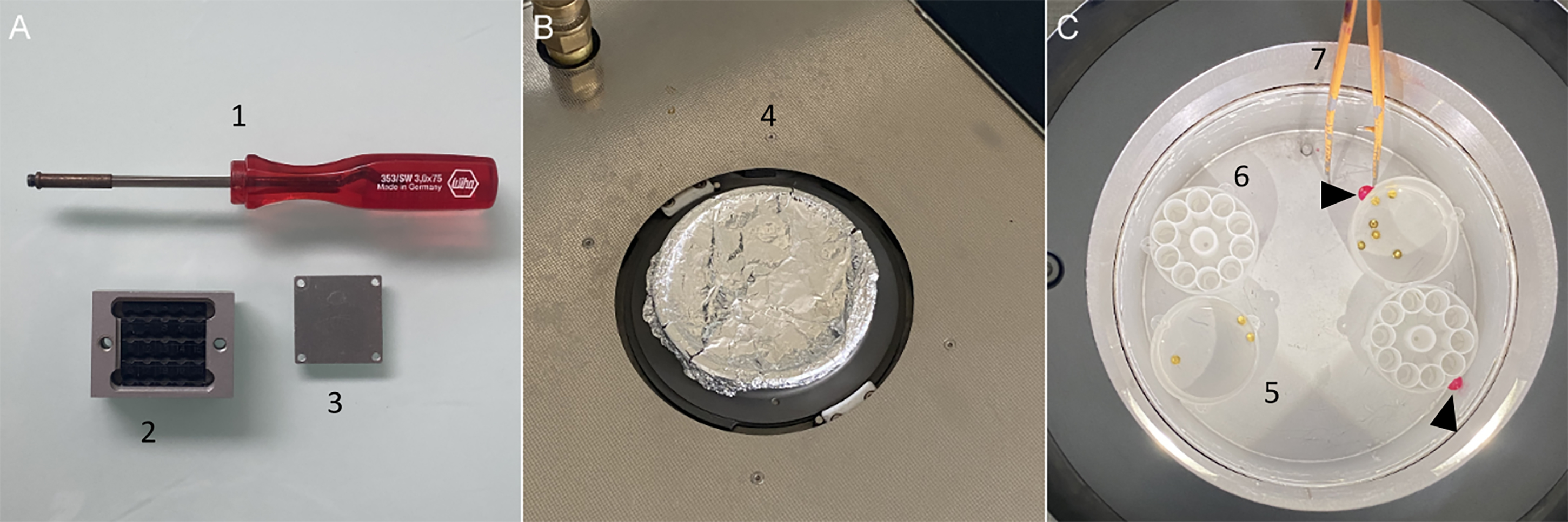
Figure 7. Freeze-substitution (FS). (A) 1. Screwdriver used to transfer; 2. Leica transfer system and 3. its lid (B) 4. Automatic FS 2 lid covered with aluminum foil. (C) 5. Leica reagent bath containing membrane carriers; 6. Flow-through ring molds; 7. Insulated pair of tweezers. Reagent bath and flow-through ring molds are labeled with nail polish to identify the different conditions (black arrowheads).Fill the AFS2 dewar with liquid nitrogen and set its temperature to -90°C. It can take more than half an hour if the device was at room temperature.
For each condition, label one reagent bath using colored nail polish and dispose them in the AFS2 chamber (Figure 7C).
Under a chemical hood and away from direct light, prepare the cryomix for FS in a glass sample vial with snap-cap (see Recipe 5). Plan to have 2.5 mL/condition. Ensure that the AFS2 light is switched off and transfer the closed vials containing the FS mix to the AFS2 chamber. By handling in the AFS2 chamber, distribute 2.5 mL of the cryomix into each reagent bath with a Pasteur pipette. Again, ensure that the AFS2 light is switched off and close its chamber by placing the lid previously covered with aluminum foil (Figure 7B). Before the following steps, ensure that the FS mix is pre-cooled by waiting at least 10 min if the AFS2 is already at -90°C.
When the temperature of the AFS2 chamber reaches -90°C, quickly transfer your frozen samples from the liquid nitrogen to the AFS2 chamber by using the pre-cooled Leica support (Figure 7A). With pre-cooled tweezers, dispatch the membrane carriers containing the frozen samples into the corresponding baths (Figure 7C). Before closing the AFS2 chamber, prepare a volume of pure acetone (plan to have 2.5 mL/per condition) in a supplemental FS bath that will be used for the next steps.
Note: If necessary, you can switch on the light of AFS2 during the handling in the AFS2 chamber. Do not forget to switch it off when handling is finished.
Set the AFS2 as follows before starting the program:
Temperature Duration -90°C 30 h +3°C/h 13 h -50°C Standby After 43 h of FS in the cryomix, when the temperature reaches -50°C, wash your samples by removing the cryomix and replacing it by 2.5 mL of pre-cooled pure acetone. Refill the supplemental FS bath without sample by a new volume of pure acetone. Wait 10 min to cool down the acetone.
Repeat the step B2.f. twice.
After the third wash with pure acetone, fill the supplemental FS bath with pure ethanol and wait 10 min for cooling down before using ethanol to wash the different samples. Repeat ethanol washes twice.
An optional step for roots, but also highly encouraged for bigger samples like hypocotyls and graft interfaces, consists of carefully separating the samples from the membrane carriers using microtools during the last ethanol wash. This step helps to optimize the resin infiltration into the biological tissues. A step-by-step guide and illustration of this procedure is described in Nicolas et al. (2018).
To free space in the AFS2 chamber, remove the supplemental reagent bath you used for rinsing. For each condition, label reagent baths plus flow-through rings using colored nail polish (Figure 7C). Place them into the AFS2. Fill them with 2.5 mL of pure ethanol and let them cool down by waiting 10 min. If you have more than two different conditions, you can sequentially add more reagent bath into the AFS2 chamber to avoid an overfilled chamber, which hampers handling.
Transfer your samples from the FS bath to one position of the plastic mold flow-through rings by pipetting the sample (it has to stay close to the tip of the pipette) with a disposable pipette of 3 mL. For samples that are kept in their carriers, use pre-cooled tweezers and place the sample on the upper face in one position of flow-through rings.
Using the AFS2 binocular, center each sample in its well of the flow-through ring with a microtool.
Under a chemical hood, prepare the first mix for the resin embedding procedure (25% of HM20 in pure ethanol) in a Leica reagent container. Plan to use 2.5 mL for each mold. Close the container before shaking it and bringing it into the AFS2 chamber for precooling. After 10 min, replace the pure ethanol in each mold by the embedding mix by slowly pipetting.
To progressively lead to a pure HM20 bath, repeat the last step for the other embedding mix (2. to 6.) following this procedure:
Mix Temperature Duration 1. HM20 25% -50°C 2 h 2. HM20 50% -50°C 2 h 3. HM20 75% -50°C overnight 4. HM20 100% -50°C 2 h 5. HM20 100% -50°C 2 h 6. HM20 100% -50°C 6 h When reaching the last embedding bath (sixth bath), mount the UV lamp and set the AFS2 as follows for the last embedding step and resin polymerization under UV:
Mix Temperature Duration HM20 100% + UV OFF -50°C 6 h HM20 100% +UV ON -50°C 24 h HM20 100% +UV ON +60°C/h ~1 h HM20 100% +UV ON 20°C 12 h Note: For thinner samples such as root tips, the third HM20 bath could be reduced to 2 h.
For our protocol, we also reduced the polymerization time under UV to limit the UV exposition of fluorescent proteins. A polymerization time of 24 h at -50°C followed by 12 h at 20°C gets resin blocks hard enough for ultramicrotomy.
Once the resin is polymerized, remove the resin blocks from the AFS2 chamber and store them in the dark in a freezer at -20°C to prevent fluorescence from photo-oxidation.
Note: For our graft interface, in samples stored for one to two years the YFP signal tends to be weak or even undetectable, while the red fluorescent protein (RFP) signal seems to be better preserved. In our opinion, to ensure the success of the CLEM approach, the processing and the observation of embedded samples should be done as quickly as possible.
Table 2. Timetable of the cryo-fixation and freeze-substitution (FS) for plant correlative light and electron microscopy (CLEM).
Ultramicrotomy
Note: During the following steps, prevent your resin block from light exposure by limiting the power of ultramicrotome light and by placing an opaque cover on your block when not sectioning. We recommend performing the sectioning step and the confocal observations on the same day to avoid a loss of the fluorescence linked to oxygen exposition of the sections. Nevertheless, if sections are prepared a few days in advance, we recommend storing them at -20°C in the dark to slow the photo-oxidation reactions.
In most cases, the conventional thickness of ultrathin sections (from 60 to 90 nm) did not allow us to detect enough fluorescent signal. In order to increase the quantity of fluorescent proteins in our sections, we increased their thickness up to 150 nm, which, in our conditions, is the optimal balance between the quantity of signal under the confocal microscope and the resolution under a 120 kV TEM. Thicker sections are less electron lucent, and the low signal-noise ratio impairs the resolution. Increasing the conventional thickness causes a loss of resolution that could be compensated by the use of a higher voltage for TEM and the electron tomography process. Note that if your fluorescence signal is very intense, you can reduce the thickness of the sections and reach a better resolution. In sum, you have to find a good balance for your samples to have enough fluorescent proteins in the section to be detected without impairing to much your final resolution on TEM.
As samples are embedded in HM20, sections need to be harvested on film-coated grids. A detailed protocol of grid filming and resin block preparation is described in Nicolas et al. (2018). We recommend working with 200 square mesh copper grids with thin bars that give a good compromise between the field of view and the robustness.
To avoid condensation on your block during sectioning, remove it from the freezer and keep it at room temperature for a few minutes in a place protected from light (a drawer for example).
Set the speed at 500 mm/s and the thickness at 500 nm on your ultramicrotome.
Trim your block with a cryotrim knife to remove the excess of resin and shape your pyramid.
When you start to cut your sample, replace the cryotrim by a histoknife. Set the speed at 1 mm/s and the thickness at 500 nm and set the cutting window with “start” and “end” on the touchscreen. Control that you reached the region of interest (ROI) by making sections of 500 nm before staining it with toluidine blue.
When the ROI is reached, replace the histoknife by an ultra-knife to make 150 nm thick sections.
Harvest sections on copper grids coated with parlodion and store in the dark until dry to ensure their perfect adhesion on the parlodion film before making microscopy observations.
Proceed to the mounting of the section between the glass slide and the coverslip.This step is delicate due to the weakness of the grids and sections. To be compatible with ulterior tomography acquisitions, grids have to be kept as flat as possible. Pay attention to manipulate the grids only on their peripheries with thin forceps. Moreover, homogeneous water immersion of the section appears to be crucial to ensure good confocal acquisitions. Take special care to avoid air bubble formation between the section and the coverslip during the grid immersion prior to the fluorescence acquisitions (Figure 8).
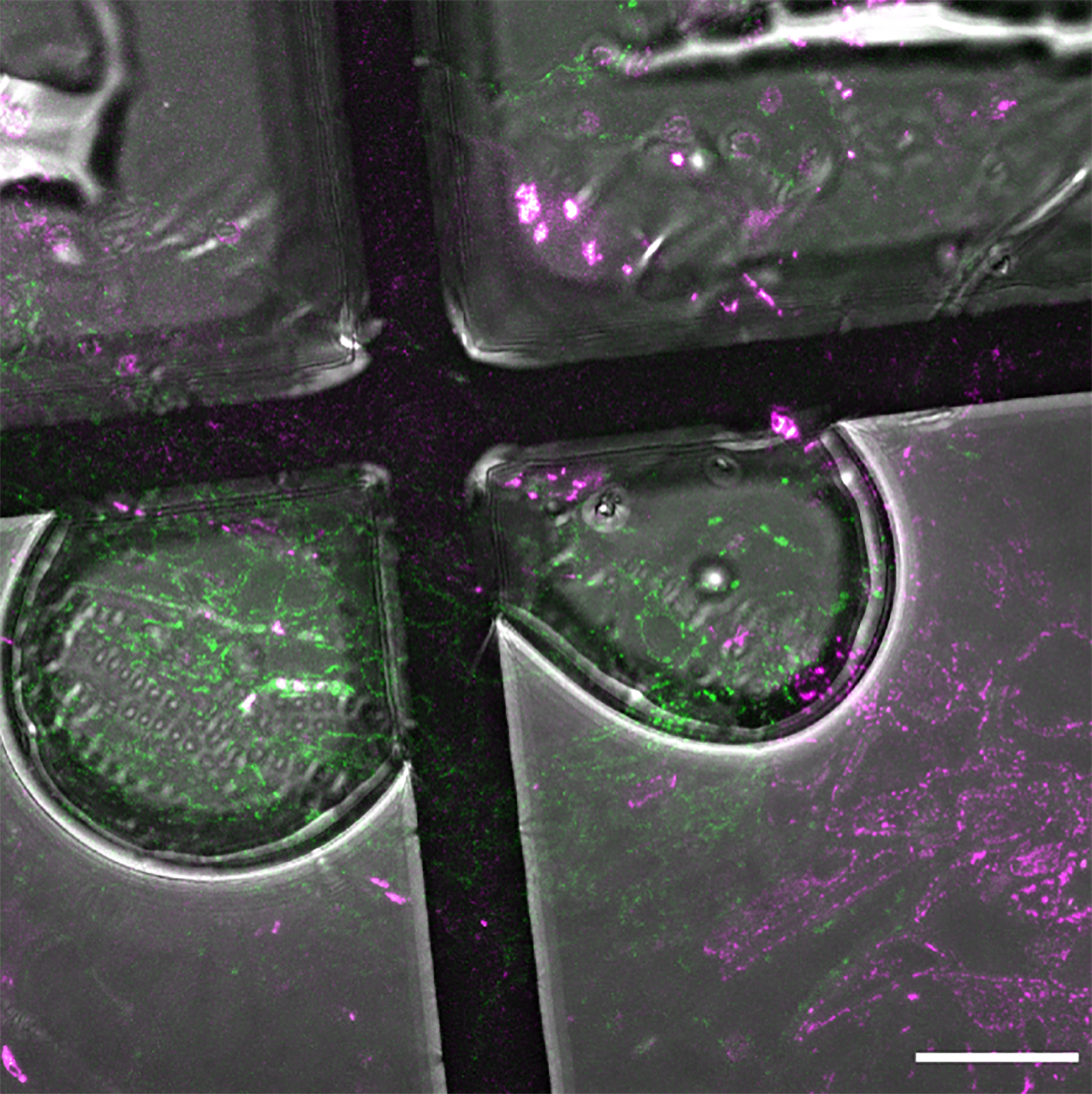
Figure 8. Air bubbles formed during the mounting step. Formation of air bubbles during the mounting can deteriorate the quality of light microscopy acquisitions due to different refraction indexes. Scale bar: 20 µm.Optional: Glow discharge
If you meet difficulties in the prevention of air bubble formation, use a glow discharger to turn the parlodion and the sections hydrophilic. Glow discharge your grids one by one just before mounting, as the effect will last only approximately 30 min.
Turn on the glow discharger system.
Clean the glow discharger chamber by doing a blank cycle: place a coverslip inside the vacuum bell and close the chamber. Close the air valve and let the pressure go down to 2 × 10⁻¹ mbar. Press the high-voltage button and adjust the voltage until the current reaches 15–20 mA. Maintain the high voltage during 30 s before gradually breaking the vacuum by opening slowly the air valve to avoid coverslip flying due to a high depressurization.
Open the vacuum bell and place the grid on the coverslip. Close the air valve and let the pressure go down to 2 × 10⁻¹ mbar. Press the high-voltage button and maintain the high voltage during 1 min. Gradually break the vacuum by opening the air valve very slowly and pick your grid up.
Mount the grids for confocal microscopy to prevent air bubbles (Figure 9A–9F, Video 2).
Video 2. Mounting the TEM grids for confocal imaging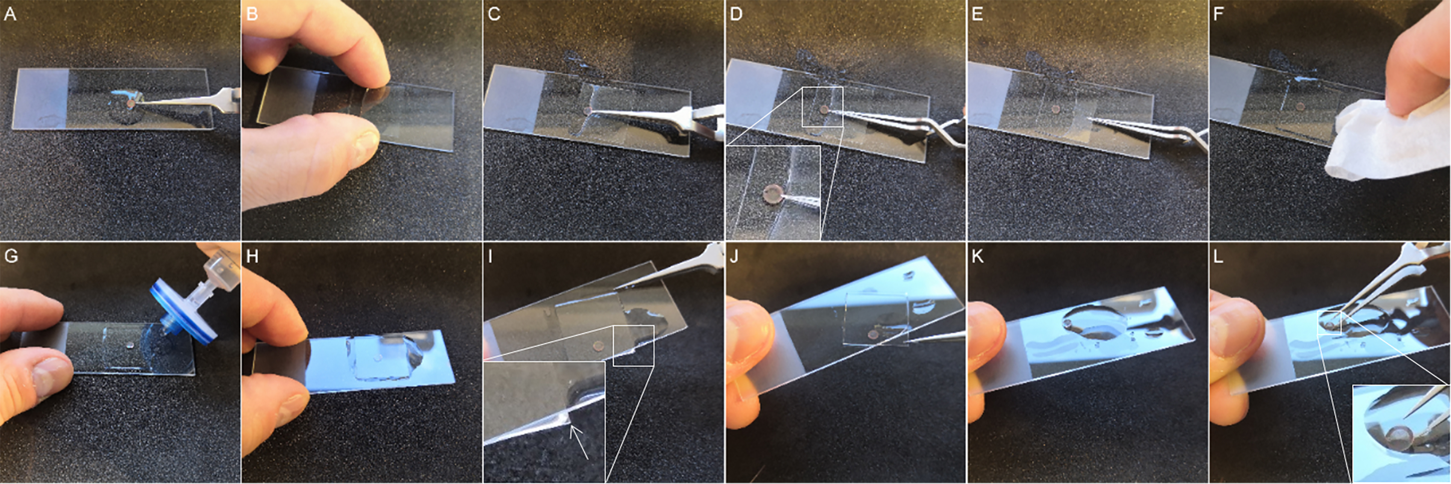
Figure 9. Mounting and unmounting of the transmission electron microscopy (TEM) grids for light microscopy (LM) observation. (A–F)Mounting of the TEM grids. (A) Prior to observation, clean the slide with ethanol to eliminate dust that can pollute the TEM grids. Then, use a syringe to put a drop of filtered water. You can wet the TEM grids on both sides so it will be easier to drop it into water later. Position the ultrathin section on the top to permit the observation of fluorescence signal even for the parts that are located on the bars of the TEM grid. (B) Approach the coverslip until it touches water. (C) Carefully place the grid between the glass slide and the coverslip with very thin tweezers. Avoid the formation of air bubbles at the surface of the grid by plunging the grid into water. (D) Release the grid from the tweezers and hold the grid in the water with the tip of the tweezers so the grid does not move when lying down the coverslip. (E) Release the grid from the tip and use the tip as a guide to slowly place the coverslip. (F) Finally, dry the excess of water with blotting paper prior to imaging. (G–L)Unmounting the TEM grids. (G and H) Add filtered water with a syringe to the side of the coverslip and wait a few minutes. (I)The excess of water helps to easily detach the coverslip from the glass slide. Slowly tilt the glass slide until a corner of the coverslip is outside the slide. (J)Remove the coverslip very carefully. At this step, there should be no resistance to avoid breaking the parlodion film. (K–L) Add more filtered water until the TEM grids unstick from the slide before taking it with the tweezers.For this step, we recommend using inverted forceps that are closed by default.
Take your grid with forceps and place the forceps on the table.
With a syringe and a 0.2 µm filter, put a drop of water on a microscope slide pre-cleaned with ethanol.
Approach a coverslip obliquely to the glass slide until it touches the water drop.
Carefully take the forceps with the grid and dip the grid into the drop of water between the slide and the coverslip. Slowly open the forceps to release the grid, which should be immersed in the water, and, with the tip of the tweezers, hold the grid in the water and lay down the coverslip on the forceps.
Remove the excess of water on the glass slide with blotting paper or paper towels. You can now place the slide under the LM and do your observations.
Confocal microscopy
During LM analyses, as the signal in the sections can be low, you could think that the fluorescence preservation failed when this is actually not the case. To detect fluorescence signal, you need to preserve and collect the maximum of photons that will be produced by your sample for your final acquisitions. In general, only one z-stack acquisition per ROI with convenient signal-noise ratio is possible for YFP. Use weak transmitted light to position you ROI in the center of the field of view rather than the fluorescent excitation source. Choose the most sensitive detector (GaAsP instead of the conventional multi-alkali photocathode) for your acquisitions. If your confocal is equipped with an AiryScan detector, it will allow you to improve the signal and the resolution. Moreover, to have the best resolution for your acquisitions, choose the objective with the highest numerical aperture (between 1.3 and 1.4) with a good fluorescence transmission and corrected to work with a coverslip. Set the larger emission window as possible to collect a maximum of emitted photons. You should have a motorized stage and consider doing Z-stack to collect the maximum of photons emitted by the section. Also, to facilitate correlation and to ensure the observation of the same region of interest, doing a tiles scan (to have an overview with good resolution) and acquiring the transmission image will help.
Start your observations through the oculars with a low magnification objective (such as 10×) with transmitted light to find and center your grid.
To localize your section more easily, close the aperture diaphragm to increase the contrast and find the edges of the section.
Increase the resolution by placing your best objective. Adjust the focus and the positioning of your sample on the stage and correctly set the aperture diaphragm (same numerical aperture as the one of the objective in place).
Shift to the confocal mode. Switch on only the mRFP excitation line and activate the detector in the transmitted position plus the most sensitive fluorescent detector. For this last one, push the signal amplification by setting the gain up to 850. Switch on only the mRFP excitation line and/or chlorophyll to preserve the maximum YFP fluorescence. Start fast-scanning to target the graft interface using the transmitted and mRFP channels and set the upper and lower Z-window limits for the Z-stack. Avoid setting a too thick Z-stack, which would induce an unproductive over-exposition of your sample.
Stop the scanning and set a sequential mode acquisition: YFP and chlorophyll on one track and mRFP on a second track. Optimize the parameters for acquisitions: pinhole opening, pixel size, z-interval, and pixel dwell time around 2 µs, and push the excitation power (up to 12% for the 488 wavelength and 3% for the 561 wavelength).
When all previous parameters are well set, start your Z-stack acquisition.
Despite the thickness of the section, not all fluorescent regions are on the same slice of the Z-stack. To facilitate the visualization, a Z-projection is systematically achieved after the Z-stack acquisition; either maximal or sum projection can work depending on your sample. Moreover, despite all efforts made for optimizing the acquisition, YFP visualization could require a compression of intensity levels of the histogram.
Removal of the EM grid (Figure 9G–9L, Video 2)
Long observations under the confocal microscope can lead to evaporation of the water between slide and coverslip, with a risk for the EM grid to stick to the glass. Taking off the coverslip when it is stuck to the glass greatly increases the chance of breaking the parlodion film.
To remove the coverslip without breaking the film, put water using a syringe (and filter) around the coverslip and wait until the coverslip is floating on water. Carefully remove the coverslip with the forceps.
If a grid is stuck to the coverslip or the glass slide, put a drop of water around the grid and wait until the grid detaches by itself and floats before taking it gently with the forceps tip.
Dry the grids by blotting it vertically on Whatman paper and put them back in the grid box for subsequent EM observations. Be sure to remember on which side of the grid your sample is, so you can observe the same side under EM (otherwise, you will have a mirror image of your sample and the correlation and localization of your region of interest will be much harder).
The fluorescence pattern observed under the confocal microscope allows the identification of cells under the EM based on their shapes.
TEM and electron tomography:
TEM observations impair molecule conformations. Fluorescence observations as well as immuno-labeling, if it is required, have to be performed systematically before the first TEM observation. For correlation, TEM overviews can be required to match the field of view of LM for correlation. Based on the shape of cells, the ROI observed with LM is targeted under TEM. To avoid miscalling and deformation during TEM acquisitions, get help from the staff of the microscopy facility to ensure the proper alignment of the TEM and the proper setting of the eucentric height. For studies that require a high ultrastructural resolution, electron tomography has to be done on the structures of interest. It allows to obtain a 3D view and to restore the loss of resolution related to thicker sections.
Only required for electron tomography:
On a parafilm strip placed on the bench, put a drop of 20 µL of the gold fiducial solution (see Recipe 9).
Put the grid of interest on the drop and let it float for 1 min.
Remove the grid with tweezers and remove the excess of gold fiducial solution remaining on the grid by carefully blotting it at its periphery with a Whatman paper.
Place the other face of the grid on the drop and let it float for 1 min before repeating step iii.
Let the grid dry before inserting it into the TEM.
Insert the grid into the TEM. Based on the cell shapes and their positions in relation to the mesh of the grid, target the ROI previously localized by LM.
Acquire a series of images to cover the integral meshes of interest with the magnification for which the objective diaphragm can be introduced. It allows you to get a complete mosaic of the ROI with enough contrast and resolution (Figure 10A).
Increase the magnification to observe your structures of interest and acquire your data. For plasmodesmata, we increased the magnification up to 41,000× and took images for intermediate magnifications to ensure success for ulterior correlations (Figure 11).
If beads were added, electron tomography acquisitions can be successfully done following the process described in the Bio-protocol paper of Nicolas et al. (2018) (Figure 11D).
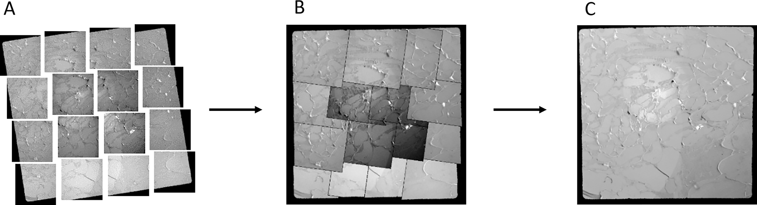
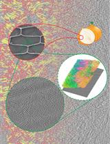
Figure 10. Mosaic acquisition and merging allows to have a large field of view for later correlation. (A) Sixteen images are acquired with the objective diaphragm on the transmission electron microscope to have a large field of view covering the graft interface. (B) Images are automatically arranged in order by the photomerge function of Adobe Photoshop. (C) Photomerge can homogenize contrast and exposure and correct geometrical deformation for a seamless fusion.
Correlation
After the acquisition of images by both LM and TEM/electron tomography, correlation of both microscopies needs to be performed to get the most out of a CLEM approach. Mosaic images (acquired at step 6c.) from TEM are fused using the photomerge function of Adobe Photoshop software (Figure 10). It permits you to have a large field of view, eventually containing the whole graft interface. At this stage, it is important to keep the raw images composing the mosaic for later analysis, as Photoshop is not able to preserve image calibration.
Correlation between LM and TEM is performed through the ec-CLEM plugin (Paul-Gilloteaux et al., 2017) of the Icy software (De Chaumont et al., 2012). On overviews, cellular landmarks that are easily recognizable in LM and TEM can be used (such as plastids, the nucleus, and cell corners, but also dirt particles) (Figure 11A). A detailed procedure and video tutorials on using ec-CLEM and Icy software are available (https://icy.bioimageanalysis.org/plugin/ec-clem/). Here is a step-by-step protocol on its use on grafted hypocotyl specimens.
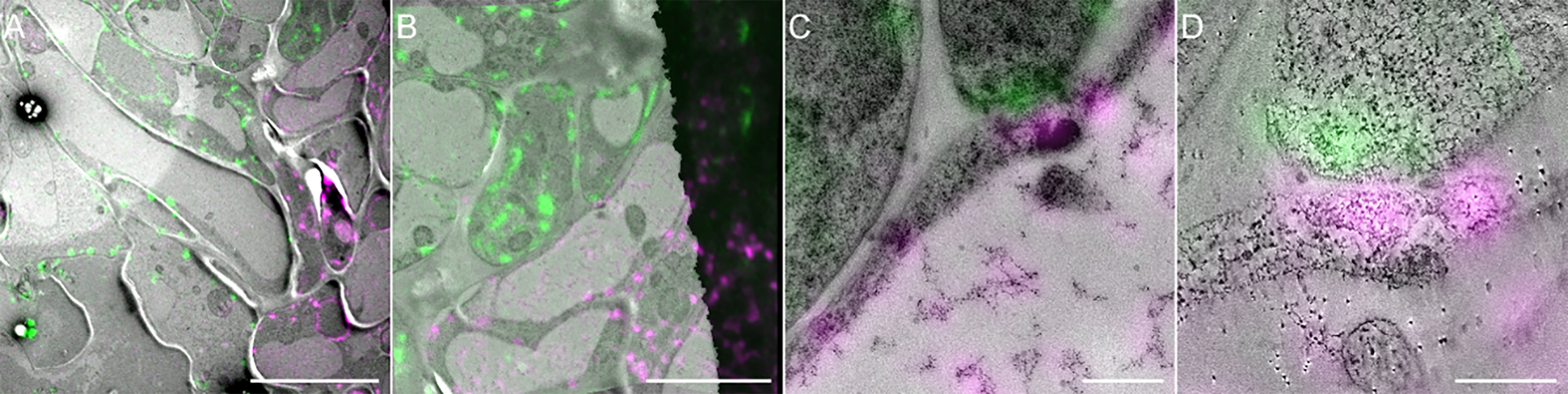
Figure 11. From correlated overview to high-resolution correlated tomogram. (A) Large CLEM field of view of a region of interest (ROI). (B) Higher magnification of the region highlighted in (A). (C) Higher magnification of the region highlighted in (B). (D) Correlated electron tomogram of the ROI corresponding to (C). Scale bars: (A) 10 µm, (B) 5 µm, (C) 0.2 µm, and (D) 0.05 µm.Copy your LM and TEM acquisitions on a new folder dedicated to the correlation where automatic xml files generated by the Icy software for automatic saving will be stored.
Open your TEM and LM images in Icy using Image > Open or by dragging and dropping your images in the software.
Once your images are open, run the ec-CLEM plugin. Set the plugin as follows: start working with “2D but let me update myself” to avoid slow process due to automatic updates of the transformation. This option is especially useful when the workstation is not powerful enough.
Select the images to process following ec-CLEM recommendations [i.e., fluorescent microscopy (FM) image to be transformed and TEM image not to be modified] and press play to run the plugin.
Place the first points on a landmark on TEM image. Adjust the position of the same landmark on the LM image. Repeat that for at least 10 points, ideally covering every region of the image, and press Update transformation . This will transform and resize the FM image based on the points you placed.
Link the two images using the lock button so their display can be synchronized to place other points more easily. Working on overviews allows you to place 10–25 markers to get a more precise correlation.
When all points are placed, update transformation again and then press the Stop button in the plugin window. This will automatically generate the correlated image that you can save. At this stage, the software may display an error message to inform you that the correlation is not perfect. This is due to anisotropic deformations linked to the HM-20 shrinkage under the electron beam.
To refine the correlation, before closing images, go back to the ec-CLEM plugin window and change the transformation to non-rigid (2D or 3D) , press play, and update transformation. Press Stop to generate the correlated image. The image generated through this method will be anisotropically transformed so each correlation point can match. You can save your image.
With the help of this correlation from overviews, TEM images at higher magnifications or electron tomography acquisitions can be used to produce high-resolution CLEM images (Figure11).
Note that correlative images are generated for visualization only and are not intended for measurement as dimension of pixel could be modified at different stages of the process (merging TEM images, correlation). If you want to measure certain characteristics of your structure of interest, such as cell wall thickness in our case, or distance between organelles for example, you have to go back to the original raw TEM images.
Data analysis
Our grafting protocol combined with HPF and our FS protocol adapted for CLEM allowed us to preserve the fluorescence of the samples together with good ultrastructural resolution. At the graft interface of A. thaliana, the origin of the cells can now be determined without any ambiguity using the expression of different fluorescent proteins for each partner (Figure 11). In comparison with standard FS with osmium tetroxide, lipidic components such as membranes are less contrasted, but still clearly visible. Moreover, if necessary, electron tomography can be applied to improve the resolution (Figure 12), as it restores the contrast quality leading to a very high resolution. Cytoplasm and plasmodesmata observed by conventional electron microscopy were indistinct, while with electron tomography they appeared much sharper, more highly contrasted, and with a higher resolution. Details such as membranes of plasmodesmata, clear ribosomes (either free or associated with the endoplasmic reticulum), and small vesicles were clearly visible. Electron tomography allowed us to reach a high 3D level of detail for the structures of interest, such as plasmodesmata, and to study their shapes in three dimensions, while this was not possible with conventional electron microscopy images (Figure 12).
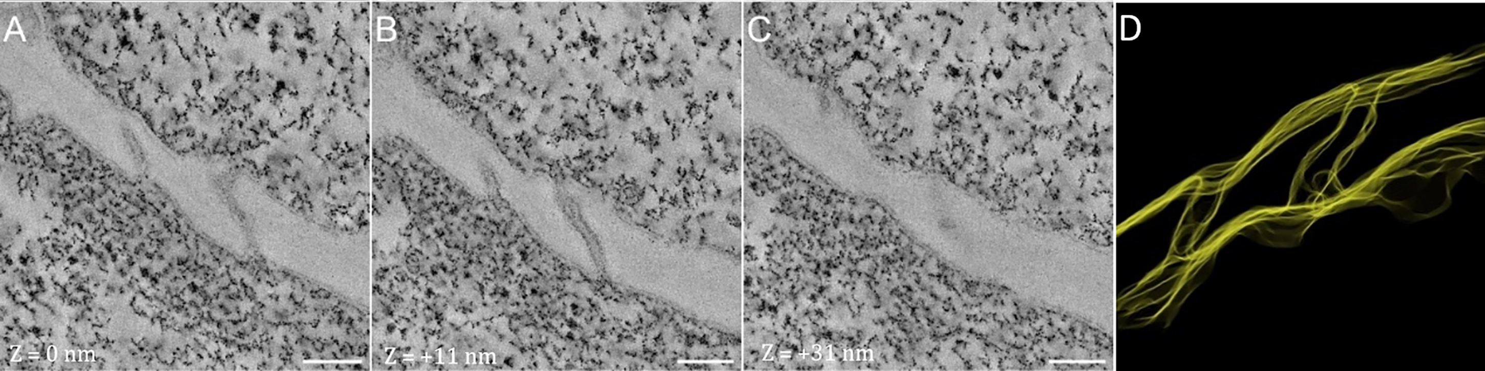
Figure 12. Electron tomography and segmentation of plasmodesmata at the graft interface. (A) Tomogram of the plasmodesmata observed at the graft interface z = 0 nm. (B) Tomogram of the PD observed at the graft interface z = + 11 nm. (C) Tomogram of the PD observed at the graft interface z = + 31 nm. (D) Segmentation of the tomograms allows the visualization of the structure in 3D. Scale bars (A–C): 100 nm.
Additionally, our protocol preserves antigenicity, thus enabling immunolabeling of desired structures for further identification under electron microscopy (Figure 13). Finally, this CLEM protocol was successfully applied on other plant tissues such as roots (Dragwidge et al., 2022; Gomez et al., 2022).
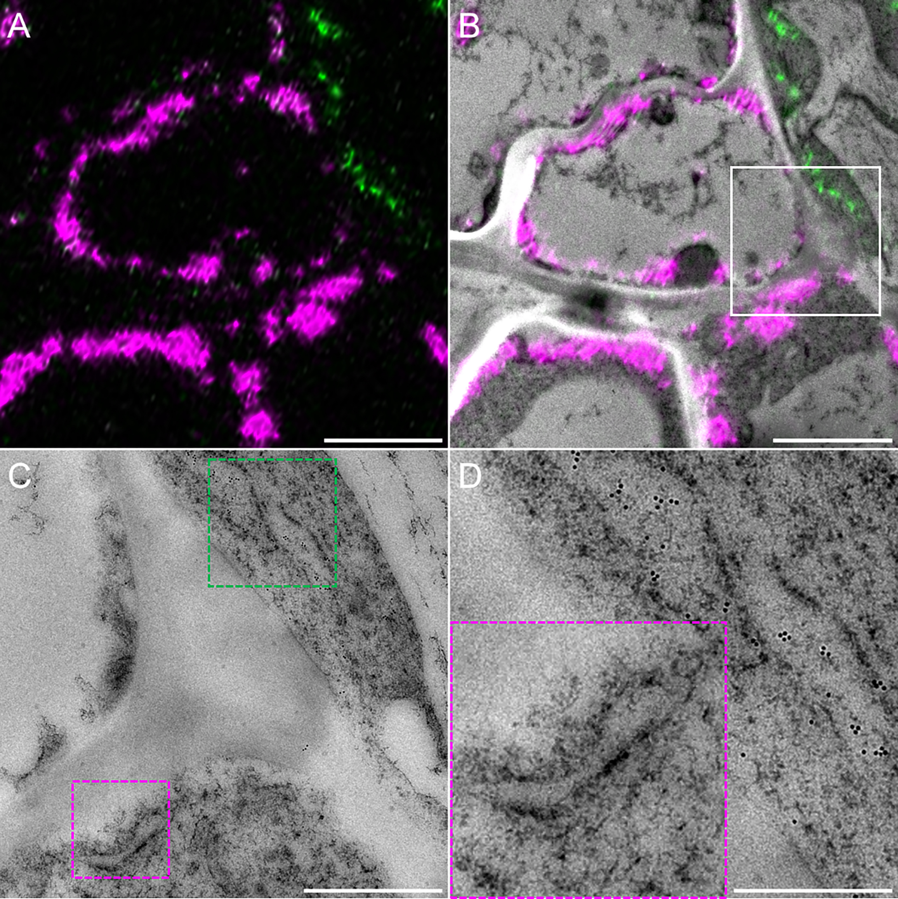
Figure 13. Immunolocalization of the yellow fluorescent protein (YFP). (A) Confocal observations of a graft interface of HDEL_YFP grafted onto HDEL_mRFP and (B) the corresponding correlated view. (C) Magnification of the region highlighted by the white square in (B), showing the endoplasmic reticulum of HDEL_mRFP (red dotted squared) and HDEL_YFP (green dotted squared). (D) Magnification of these regions reveal the presence of the endoplasmic reticulum immunolabeled with gold particles for HDEL_YFP cell, while there are no gold particles in the endoplasmic reticulum of HDEL_mRFP cell. Scale bars: (A and B) 3 µm, (C) 1 µm, (D) 500 nm.
Notes
When doing the seed sterilization, you need to work with bleach and acid separately to prevent an accidental mix of the two reagents. Always use the appropriate protective equipment as gloves and a lab coat.
Recipes
Bleach solution for seeds sterilization
Dissolve one tablet (containing 1.5 g of active bleach) in 50 mL of distilled water (3% w/v in active bleach)
Culture media for seedlings and grafting
Half-strength MS medium for seedlings (1 L)
MS medium + vitamins: 2.2 g
Plant agar: 8 g
Adjust pH with 1 N KOH solution to 5.8
Autoclave flasks at 120°C for 20 min
Water medium for grafting
Volume (mL) 100 200 300 40 500 1,000 Approximate number of Petri dishes 5 10 15 20 25 50 Agar (g) 1.6 3.2 4.8 6.4 8 16 Adjust pH with 1 N KOH solution to 5.8.
Autoclave flasks at 120°C for 20 min
Put the autoclaved medium in the Petri dishes while it is still hot and liquid. Prepare only the amount of medium you need, according to the planned number of grafts.
20% BSA solution for cryoprotection during HPF
Weigh 0.4 g of BSA and put it into a 2 mL screw-top sample tube.
Complete with water (or your medium culture) up to 2 mL.
Altern quick centrifugations and vortex until BSA is dissolved entirely.
If necessary, complete with water up to 2 mL to get a final concentration of 20%.
Cryosubstitution uranyl-acetate stock solution (20%, 500 µL)
Weigh 0.1 g of uranyl acetate powder (gloves and dust mask required) and put in a 2 mL screw-cap tube.
Add pure methanol (under a ventilated hood) up to 500 µL.
Wrap the tube in tinfoil and store in the dark at -20°C in a dedicated cryosubstitution box.
Cryosubstitution mix for 3 mL
Compound (initial concentration) Volume (mL) Final concentration Uranyl acetate powder (20% w/v in pure methanol) 0.015 0.1% Pure acetone 2.985 - HM20 solutions
Make the solution in the FS Leica plastic solvent container and cool it for 10–15 min in AFS chamber before use.
HM20 concentration HM20 volume (mL) Pure ethanol (mL) 20% 2 8 50% 5 5 75% 7.5 2.5 2% parlodion solution for grid filming
Prepare only a small quantity of parlodion in a small glass flask, as it is very sensitive to humidity and will not preserve properly over a long time.
Weigh a small piece of solid parlodion (approximately 0.01 g) after cutting.
Add isoamyl-acetate (store in a vented solvent cupboard and keep away from humidity) up to 1 mL.
Wrap the flask in tinfoil and seal the lid with Parafilm.
Before first use, agitate to homogenize the solution. Always seal the lid and protect from light.
Toluidine blue solution
Make a stock solution with 1 g of toluidine blue powder and 1 g of sodium borate in 20 mL of distilled water.
Dilute 25 times to prepare the working solution.
Gold fiducial solution
Make a solution of 0.5% BSA in MilliQ water.
Filtrate the solution with a 0.2 µm filter connected to a syringe.
Mix colloidal gold solution in 0.5% BSA (1:1 ratio). Aliquot in 0.5 mL sample tubes and store at -20°C.
Acknowledgments
The Ph.D. thesis of C.C. was financed by grants entitled “Etude des mécanismes de l’union greffon /porte-greffe,” 50% from the French National Institute for Agronomical Research/INRAE department “Plant biology and breeding/BAP” and 50% from the Région Nouvelle Aquitaine, France. Further financial support was provided by the Starter grant “Etude des mécanismes de l’union greffon/porte-greffe” also from BAP. The Institute of Vine and Wine Science (ISVV) supported a travel grant for C.C. to go to Charles Melnyk’s lab to learn grafting procedure. Thanks to Charles Melnyk and Remi Lemoine who invited me to learn the grafting procedure of A. thaliana . This project has received funding from the European Research Council (ERC) under the European Union’s Horizon 2020 research and innovation program (grant agreement No 852136 to AB). All sample preparation and imaging was done on the Pôle Imagerie du Végétale, from Bordeaux Imaging Centre (http://www.bic.u-bordeaux.fr/).
Competing interests
The authors declare to have no competing interest
References
- Bell, K., Mitchell, S., Paultre, D., Posch, M. and Oparka, K. (2013). Correlative imaging of fluorescent proteins in resin-embedded plant material. Plant Physiol 161(4): 1595-1603.
- Bidadi, H., Matsuoka, K., Sage-Ono, K., Fukushima, J., Pitaksaringkarn, W., Asahina, M., Yamaguchi, S., Sawa, S., Fukuda, H., Matsubayashi, Y., et al. (2014). CLE6 expression recovers gibberellin deficiency to promote shoot growth in Arabidopsis. Plant J 78(2): 241-252.
- Chambaud, C., Cookson, S. J., Ollat, N., Bayer, E. and Brocard, L. (2022). A correlative light electron microscopy approach reveals plasmodesmata ultrastructure at the graft interface. Plant Physiol 188(1): 44-55.
- De Chaumont, F., Dallongeville, S., Chenouard, N., Herve, N., Pop, S., Provoost, T., Meas-Yedid, V., Pankajakshan, P., Lecomte, T., Le Montagner, Y., et al. (2012). Icy: an open bioimage informatics platform for extended reproducible research. Nat Methods 9(7): 690-696.
- Dean, N. and Pelham, H. R. (1990). Recycling of proteins from the Golgi compartment to the ER in yeast. J Cell Biol 111(2): 369-377.
- Dragwidge, J. M., Wang, Y., Brocard, L., De Meyer, A., Hudeček, R., Eeckhout, D., Chambaud, C., Pejchar, P., Potocký, M., Vandorpe, M., et al. (2022). AtEH/Pan1 proteins drive phase separation of the TPLATE complex and clathrin polymerisation during plant endocytosis. BioRxiv, 2022.03.17.484738.
- Gautier, A. T., Chambaud, C., Brocard, L., Ollat, N., Gambetta, G. A., Delrot, S. and Cookson, S. J. (2019). Merging genotypes: graft union formation and scion-rootstock interactions. J Exp Bot 70(3): 747-755.
- Gomez, R. E., Chambaud, C., Lupette, J., Castets, J., Pascal, S., Brocard, L., Noack, L., Jaillais, Y., Joubes, J. and Bernard, A. (2022). Phosphatidylinositol-4-phosphate controls autophagosome formation in Arabidopsis thaliana. Nat Commun 13(1): 4385.
- Lindsey, B. E., 3rd, Rivero, L., Calhoun, C. S., Grotewold, E. and Brkljacic, J. (2017). Standardized Method for High-throughput Sterilization of Arabidopsis Seeds. J Vis Exp(128): 56587.
- Knox, K., Wang, P., Kriechbaumer, V., Tilsner, J., Frigerio, L., Sparkes, I., Hawes, C. and Oparka, K. (2015). Putting the Squeeze on Plasmodesmata: A Role for Reticulons in Primary Plasmodesmata Formation. Plant Physiol 168(4): 1563-1572.
- Kollmann, R. and Glockmann, C. (1985). Studies on graft unions. I. Plasmodesmata between cells of plants belonging to different unrelated taxa. Protoplasma 124(3): 224-235.
- Kollmann, R. and Glockmann, C. (1991). Studies on graft unions - III. On the mechanism of secondary formation of plasmodesmata at the graft interface. Protoplasma 165(1-3): 71-85.
- Kollmann, R., Yang, S. and Glockmann, C. (1985). Studies on graft unions - II. Continuous and half plasmodesmata in different regions of the graft interface. Protoplasma 126(1-2): 19-29.
- Kremer, J. R., Mastronarde, D. N. and McIntosh, J. R. (1996). Computer visualization of three-dimensional image data using IMOD. J Struct Biol 116(1): 71-76.
- Kukulski, W., Schorb, M., Kaksonen, M. and Briggs, J. A. (2012a). Plasma membrane reshaping during endocytosis is revealed by time-resolved electron tomography. Cell 150(3): 508-520.
- Kukulski, W., Schorb, M., Welsch, S., Picco, A., Kaksonen, M. and Briggs, J. A. (2012b). Precise, correlated fluorescence microscopy and electron tomography of lowicryl sections using fluorescent fiducial markers. Methods Cell Biol 111: 235-257.
- Lee, H., Sparkes, I., Gattolin, S., Dzimitrowicz, N., Roberts, L. M., Hawes, C. and Frigerio, L. (2013). An Arabidopsis reticulon and the atlastin homologue RHD3-like2 act together in shaping the tubular endoplasmic reticulum. New Phytol 197: 481-489.
- Marion, J., Le Bars, R., Satiat-Jeunemaitre, B. and Boulogne, C. (2017). Optimizing CLEM protocols for plants cells: GMA embedding and cryosections as alternatives for preservation of GFP fluorescence in Arabidopsis roots. J Struct Biol 198(3): 196-202.
- Melnyk, C. W. (2017a). Grafting with Arabidopsis thaliana. Methods Mol Biol 1497: 9-18.
- Melnyk, C. W. (2017b). Monitoring Vascular Regeneration and Xylem Connectivity in Arabidopsis thaliana. Methods Mol Biol 1544: 91-102.
- Melnyk, C. W., Gabel, A., Hardcastle, T. J., Robinson, S. and Miyashima, S. (2018). Transcriptome dynamics at Arabidopsis graft junctions reveal an intertissue recognition mechanism that activates vascular regeneration.PNAS 115(10). https://doi.org/10.1073/pnas.1718263115.
- Melnyk, C. W., Schuster, C., Leyser, O. and Meyerowitz, E. M. (2015). A Developmental Framework for Graft Formation and Vascular Reconnection in Arabidopsis thaliana. Curr Biol 25(10): 1306-1318.
- Molnar, A., Melnyk, C. W., Bassett, A., Hardcastle, T. J., Dunn, R. and Baulcombe, D. C. (2010). Small silencing RNAs in plants are mobile and direct epigenetic modification in recipient cells. Science 328(5980): 872-875.
- Mudge, K. (2009). A History of Grafting. Horticultural Reviews 35: 437-494.
- Nelson B. and Nebenführ (2007). A multicolored set of in vivo organelle markers for co-localization studies in Arabidopsis and other plants. Plant J 51:1126-1136.
- Nicolas, W. J., Bayer, E. and Brocard, L. (2018). Electron Tomography to Study the Three-dimensional Structure of Plasmodesmata in Plant Tissues-from High Pressure Freezing Preparation to Ultrathin Section Collection. Bio-protocol 8(1): e2681.
- Notaguchi, M., Kurotani, K. I., Sato, Y., Tabata, R., Kawakatsu, Y., Okayasu, K., Sawai, Y., Okada, R., Asahina, M., Ichihashi, Y., et al. (2020). Cell-cell adhesion in plant grafting is facilitated by b-1,4-glucanases.Science 369(6504): 698-702.
- Paul-Gilloteaux, P., Heiligenstein, X., Belle, M., Domart, M. C., Larijani, B., Collinson, L., Raposo, G. and Salamero, J. (2017). eC-CLEM: flexible multidimensional registration software for correlative microscopies. Nat Methods 14(2): 102-103.
- Pina, A., Cookson, S. J., Calatayud, A., Trinchera, A. and Errea, P. (2017). Physiological and molecular mechanisms underlying graft compatibility. Chapter 5. Vegetable Grafting. Principles and Practices. 132-154.
- Studer, D., Graber, W., Al-Amoudi, A. and Eggli, P. (2001). A new approach for cryofixation by high-pressure freezing. J Microsc 203(Pt 3): 285-294.
- Turnbull, C. G. N. (2010). Grafting as a Research tool. Methods Mol Biol 655: 11-26.
- Turnbull, C. G., Booker, J. P. and Leyser, H. M. (2002). Micrografting techniques for testing long-distance signalling in Arabidopsis. Plant J 32(2): 255-262.
- Wu, R., Wang, X., Lin, Y., Ma, Y., Liu, G., Yu, X., Zhong, S. and Liu, B. (2013). Inter-species grafting caused extensive and heritable alterations of DNA methylation in Solanaceae plants. PLoS One 8(4): e61995.
- Yang, Y., Mao, L., Jittayasothorn, Y., Kang, Y., Jiao, C., Fei, Z. and Zhong, G.-Y. (2015). Messenger RNA exchange between scions and rootstocks in grafted grapevines.BMC Plant Biology 15(1): 251.
- Zhang, W., Kollwig, G., Stecyk, E., Apelt, F., Dirks, R. and Kragler, F. (2014). Graft-transmissible movement of inverted-repeat-induced siRNA signals into flowers.Plant J 80(1): 106-121.
Article Information
Copyright
© 2023 The Authors; exclusive licensee Bio-protocol LLC.
How to cite
Chambaud, C., Cookson, S. J., Ollat, N., Bernard, A. and Brocard, L. (2023). Targeting Ultrastructural Events at the Graft Interface of Arabidopsis thaliana by A Correlative Light Electron Microscopy Approach. Bio-protocol 13(2): e4590. DOI: 10.21769/BioProtoc.4590.
Category
Plant Science > Plant physiology > Tissue analysis
Cell Biology > Cell imaging > Electron microscopy
Do you have any questions about this protocol?
Post your question to gather feedback from the community. We will also invite the authors of this article to respond.