- Protocols

- Articles and Issues
- For Authors
- About
- Become a Reviewer

Focused Ion Beam Milling and Cryo-electron Tomography Methods to Study the Structure of the Primary Cell Wall in Allium cepa

Published: Vol 12, Iss 23, Dec 5, 2022 DOI: 10.21769/BioProtoc.4559 Views: 2586
Reviewed by: Shyam SolankiAnonymous reviewer(s)
Original research article
The authors used this protocol in:
Jun 2022
Advertisement


Protocol Collections
Comprehensive collections of detailed, peer-reviewed protocols focusing on specific topics


Abstract
Cryo-electron tomography (cryo-ET) is a formidable technique to observe the inner workings of vitrified cells at a nanometric resolution in near-native conditions and in three-dimensions. One consequent drawback of this technique is the sample thickness, for two reasons: i) achieving proper vitrification of the sample gets increasingly difficult with sample thickness, and ii) cryo-ET relies on transmission electron microscopy (TEM), requiring thin samples for proper electron transmittance (<500 nm). For samples exceeding this thickness limit, thinning methods can be used to render the sample amenable for cryo-ET. Cryo-focused ion beam (cryo-FIB) milling is one of them and despite having hugely benefitted the fields of animal cell biology, virology, microbiology, and even crystallography, plant cells are still virtually unexplored by cryo-ET, in particular because they are generally orders of magnitude bigger than bacteria, viruses, or animal cells (at least 10 μm thick) and difficult to process by cryo-FIB milling. Here, we detail a preparation method where abaxial epidermal onion cell wall peels are separated from the epidermal cells and subsequently plunge frozen, cryo-FIB milled, and screened by cryo-ET in order to acquire high resolution tomographic data for analyzing the organization of the cell wall.
Keywords: FIB-millingBackground
Cryo-electron tomography (cryo-ET) relies on the ability to observe a thin vitrified or cryo-immobilized sample. Vitrified water is a metastable state of water achieved when the freezing rate is high enough that the water molecules do not have time to reorganize in a hexagonal lattice crystal (Dubochet, 2007). This state of water, also called amorphous ice, can also withstand the vacuum of the cryo-electron microscope (cryo-EM). In turn, the sample is observed in a near-native state, as all cellular processes were immobilized at freezing time. At ambient pressure, vitrification is achieved by plunge freezing the sample in liquid propane, ethane, or a mix of both. The freezing rates achievable with these cryogens at ambient pressure limit vitrification thickness to approximately 10 μm. After proper vitrification, samples that exceed 500 nm in thickness need to be thinned down. The go-to method nowadays is cryo-focused ion beam (cryo-FIB) milling (Villa et al., 2013). Originally used in the material science field, this technique uses a focused gallium beam to erode the sample away and create thin lamellae, approximately 200 nm thick, amenable to cryo-ET.
Onion epidermal cell wall peels have been used in atomic force microscopy (AFM) studies to study the arrangement of the cellulose fibers in the superficial inner layers of the cell wall (Kafle et al., 2013; T. Zhang et al., 2014, 2017). They are a model for the structural and mechanical study of the primary cell wall (Y. Zhang et al., 2021). Despite being a high-resolution imaging method allowing observations in the native state, AFM can only image the few superficial layers of the cell wall. These cell wall peels happen to be between 5 and 10 μm in thickness, which is compatible with plunge freezing but still too thick for direct imaging by cryo-EM. Performing cryo-FIB milling on the cell wall peels allow i) screening and tilt series acquisition by cryo-ET, and ii) access to the deeper layers of the cell wall, previously unattainable by AFM. This protocol describes the sample preparation, data acquisition, and processing involved in our study called “Cryo-electron tomography of the onion cell wall shows bimodally oriented cellulose fibers and reticulated homogalacturonan networks” (Nicolas et al., 2022). We are confident that this system, in conjunction with cryo-ET and cryo-FIB milling, can become a powerful method to study the effects of mechanical stress and various treatments on the cell wall, while allowing a better understanding of the interaction of the different components present in the cell wall and their mechanical impact there.
Materials and Reagents
Plant material
Plastic Petri dishes (RPI, catalog number: 160265)
Sharp knife
Double edge razor blades (EMS, catalog number: 72002-01)
Glass slides (EMS, catalog number: 71863-01)
Cover slips (VWR, catalog number: 48366-067)
Fresh white onions from the local supermarket (see Note 1)
HEPES powder (RPI, catalog number: H75030-50.0)
CAPS powder (Sigma, catalog number: C2632-100G)
KOH powder (Sigma, catalog number 06103-1KG)
Tween-20 (RPI, catalog number: P20370-0.5)
Deionized (DI) water
BAPTA (Sigma-Aldrich, catalog number: C2632-100)
Pectate lyase from Aspergillus (Megazyme, catalog number: E-PCLYAN2)
NaOH powder (Sigma, catalog number RDD007-1KG)
HEPES 20 mM buffer solution (see Recipes)
CAPS 50 mM buffer solution (see Recipes)
Pectate lyase at 4.7 U/mL (5 mL) (see Recipes)
BAPTA 2 mM (see Recipes)
Plunge freezing
Glass slides (EMS, catalog number: 71863-01)
Grid boxes (Thermo Fisher) (see Note 2)
London Finder Quantifoil grids NH2 R2/2 copper 200 mesh (EMS #LFH2100CR2) (see Note 3)
Cut up blotting pads (Whatman, catalog number: 1540-055)
Liquid nitrogen
Liquid ethane/propane (60/40 ratio)
Ethanol 70%
Grid clipping
FIB autogrids (Thermo Fisher, catalog number: 1205101)
C-rings (Thermo Fisher)
Magnifying lens (Intertek LTS-F21-61)
Clipping pens (Thermo Fisher)
Sharpie pen (red or black)
Autogrid grid boxes (Thermo Fisher)
Lid pen (Thermo Fisher)
Cryo-FIB milling
Liquid nitrogen
Argon gas
Shuttle (Quorum Tech, catalog number: 12406)
Cryo-ET screening and tilt-series acquisition
Grid cassette (Thermo Fisher)
NanoCab (Thermo Fisher)
Equipment
Plant material
Any light microscope equipped with phase contrast
Plunge freezing
EMS tweezers (EMS style 2, 5, 3X, and 7)
Vitrobot tweezers (Inox-Medical LS 11253-27)
Flexible LED lamp
Large forceps and small rubber band (EMS style 7330)
Vitrobot Mark II (Thermo Fisher)
Glow discharger (EMS 100X, not sold anymore; alternatively, Pelco easyGlow)
Liquid nitrogen storage system (Worthington HC35)
LN2 containers (spearlab.com)
Grid clipping
Autogrid tweezers (PELCO 5046-SV)
Clipping station (Thermo Fisher)
Cryo-FIB milling
Versa 3D DualBeam FIB-SEM (FEI)
Quorum PP3000T transfer system (Quorum Tech)
Cryo-ET screening and tilt series acquisition
Titan Krios 300 kV microscope (Thermo Fisher)
Gatan K3 direct director (Gatan)
Post-column GIF energy filter (Thermo Fisher)
Software
SerialEM (https://bio3d.colorado.edu/) (Mastronarde, 2003, 2005), to control the TEM
Gatan DM3 (https://www.gatan.com/products/tem-analysis/gatan-microscopy-suite-software), to control the K3 detector
Etomo (https://bio3d.colorado.edu/imod/download.html) for tomogram reconstruction and 3dmod for tomogram visualization (Kremer et al., 1996; Mastronarde, 1997; Mastronarde and Held, 2017)
EMAN2 (https://blake.bcm.edu/emanwiki/EMAN2) for Convolutional Neural Network (CNN) training and application (Chen et al., 2017; Tang et al., 2007, p. 2), Amira and the Xtracing plugin (Thermo Fisher) (https://www.thermofisher.com/us/en/home/electron-microscopy/products/software-em-3d-vis/amira-software.html) for segmentation (Rigort et al., 2012)
ARETOMO for automated alignment and reconstruction (https://msg.ucsf.edu/software)
Custom scripts derived from Dimchev et al. (2021)
R and R studio to analyze the data (https://cran.r-project.org/index.html, https://www.rstudio.com/)
Procedure
Preparation of the onion cell wall peels
Note: This protocol involves the use of liquid nitrogen and other cryogenic liquids that could lead to severe burning if not handled properly. Please refer to your institution’s safety guidelines for manipulation of these liquids. For all the following steps described in this manuscript, samples after vitrification should always be handled with pre-cooled tools, so always precool the tools before touching the grids or grid boxes to avoid devitrification of the sample.
Gather fresh, hard, hydrated white onions (see Note 1).
Cut off the tips of the onion and take off the dried, brownish superficial layers until the first fresh layer is reached (Video 1, step 1). This is layer one (Figure 1A).
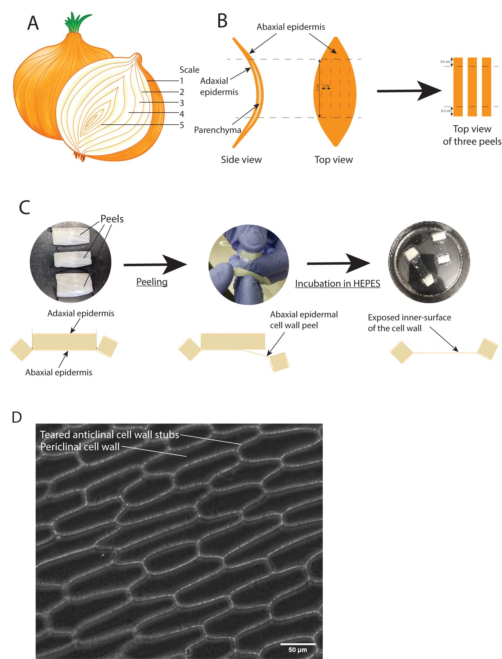
Figure 1. Anatomy of an onion scale and generation of the epidermal cell wall peels. (A) Global view of a longitudinally cut onion. (B) Side and top views (left and middle, respectively) of an onion scale. Black lines indicate the first incisions to be done to cut away the tips. Red lines indicate the incisions to be done to create the rectangular cell wall peels. Right, top view of three separate rectangular-like scale explants with the black lines indicating the incisions to be made to create handles that will be used to generate the peels in the next step. (C) Top row: left shows top views of three rectangular-like scale explants. Here, the abaxial epidermis is facing upwards (glowing, waxy side) and is the side to be used to generate the cell wall peel. Middle shows a piece of onion scale in the process of being peeled. The clear membrane is the cell wall peel. Right shows two cell wall peels with the two handles at their extremity incubating in HEPES buffer. Bottom row: side view diagrams of the peeling process. Left shows a scale just incised, so that the abaxial epidermal layer has not been cut (black dashed lines). The two side squares are the handles to pull on in order to create the cell wall peel. Middle shows the beginning of the process where the handle is pulled away from the main body of the scale to tear away the abaxial epidermal layer. Right shows the epidermal peel where the abaxial epidermal cells were ripped in half. The two handles on the side are used to manipulate the peel. (D) Contrast phase image of a successfully peeled abaxial epidermal cell wall. The anticlinal cell walls show jagged edges. See also Video 1. Video 1. Peeling of the onion.
The peeling procedure to create the cell wall peels from intact onions is described; it is divided into five steps: i) preparation of the onion, ii) sampling the scales, iii) preparing the scales, iv) peeling the cell wall, and v) screening of the cell wall peel.Create two deep longitudinal incisions going down to the core of the onion. These incisions should cover approximately a quarter of the onion (90°) (Video 1, step 2).
Take apart the scales from this excised part. The scales are concave (Figure 1B) and the abaxial side, where the peels will be created, faces outside (convex part). Keep note of the order of the scales.
Cut off the tips of the scale (a few centimeters from the tips) and keep the central large part of the scale (Figure 1B, black dashed lines, and Video 1, step 3).
Cut this central part longitudinally in several bands, each approximately 3 cm long and 1 cm wide (Figure 1B, red dashed lines, and Video 1, step 3). There should now be several rectangular excisions from the scale (3 × 1 cm). The waxy, hydrophobic side is the epidermis and the more porous side will be discarded later.
For each band, create two transversal incisions 0.5 cm away from the extremities on the adaxial porous side. These incisions should go through the entire scale, except the waxy abaxial thin membrane, i.e., the epidermal cell wall (Figure 1B and C and Video 1, step 4). The excised scales should now have two floppy extremities, here called handles (Video 1, step 4).
Grab one of the handles, fold over towards the epidermal cell wall and pull by brief powerful strokes to rip the abaxial epidermal cells in half. A Velcro sound should be heard (Video 1, step 4).
A continuous membrane between the two thick handles indicates successful cell wall peeling (Figure 1C).
Cut off one of the handles and mount the peel between glass slide and cover slip. Screen the peel by light microscopy to control its quality. Only peels with close to 100% ripped cells are kept for freezing (Figure 1D, Video 1, step 5).
Incubate the peels in HEPES 20 mM buffer (see Recipe 1) for 20 min to clean out cellular remnants off the cell wall peel.
Plunge freezing of the cell wall peels
Note: The onion cell wall peels need to be presented parallel to the FIB beam for optimal milling. It is therefore important to keep track of the direction of the cells within the peel during freezing, clipping, and mounting of the grids in the FIB-SEM, despite not being able to see the cells (see Note 4).
Turn on the Vitrobot and prepare the liquid nitrogen and ethane/propane cup (Video 2, step 1).
Video 2. Plunge freezing of the cell wall peels.
The cell wall peel vitrification procedure is described: i) preparing the freezing well, ii) glow discharging the grids, iii) cutting up the cell wall peel to fit on an EM grid, iv) setting the cell wall peel explant on the EM grid, and v) grid blotting and plunge freezing.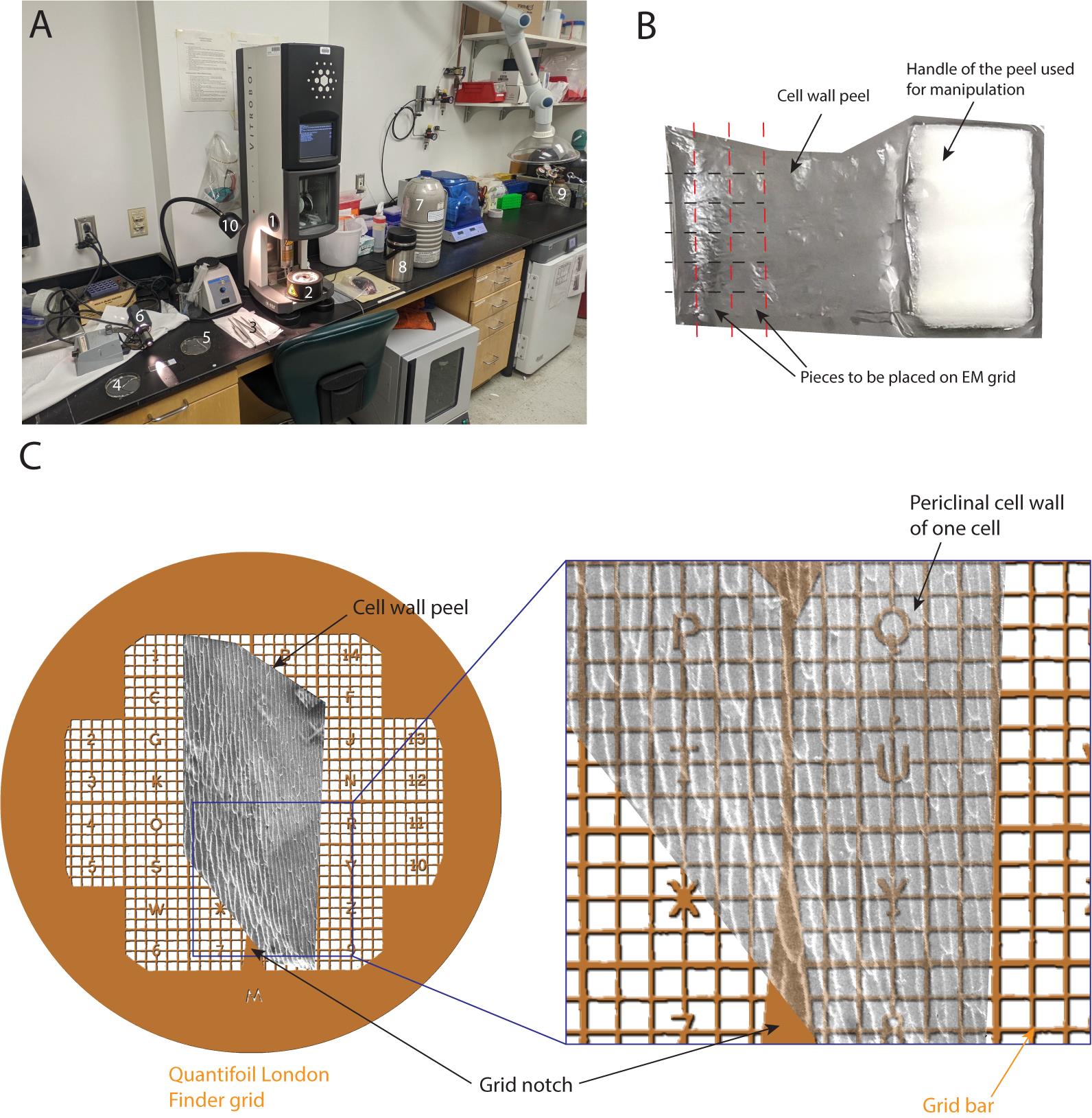
Figure 2. Plunge freezing of the cell wall peels. (A) Global view of the freezing setup: 1- Vitrobot, 2- Freezing well, 3- Various tweezers and forceps, 4- Petri dish with HEPES buffer and cell wall peels, 5- Glass slide where the cell wall peel will be dissected, 6- Light shining tangential to the table, 7- Liquid nitrogen dewar, 8- Liquid nitrogen container for grid boxes, 9- Propane/ethane filling station, and 10- Desk lamp shining at the well for extra visibility while transferring vitrified grids to the grid boxes. (B) Top view of a cell wall peel, where one handle (left one) has been removed. Black dashed lines indicate the first incisions to be made. Red dashed lines indicate the latter incisions to be made to generate small rectangles to be positioned on the EM grid. (C) Top view of a London Finder Quantifoil grid with a cell wall peel positioned along the grid notch. The right inset shows that the long axis of the onion cells is more or less parallel to the direction of the main notch. See also Video 2.Glow-discharge the grids at 20 mA for 1 min (Video 2, step 2).
Gather all necessary tools and equipment to prepare the rectangles of the cell wall next to the plunge freezer (Figure 2A).
Prepare labeled grid boxes (see Note 2) and long forceps with blotting pad at the end.
Place the cell wall peel on a glass slide with a drop of HEPES buffer. Never let the peel dry out.
Shine a bright light tangential to the glass slide towards the experimenter in order to see the edges of the thin cell wall peel (Video 2, step 3).
Optionally, if certain extremities of the peel look sub-optimal, cut and discard them, so that the region to be used is accessible now.
Use the Vitrobot tweezers to securely grab the Quantifoil EM grid at the triangular notch (Figure 2C shows the Quantifoil notch, Video 2, step 3).
Using a sharp razor blade, apply constant pressure on the peel extremity to make clean incisions, parallel to the long side of the peel, approximately 1 cm long if possible. Reiterate this process on the whole width of the peel in order to have clean parallel incisions equal in length (Figure 2B black dashed lines, Video 2, step 3).
Make clean incisions perpendicular to the ones generated in step B9 starting on one side of the peel. This will free a small rectangle of approximately 3 × 1 mm that can fit on an EM Quantifoil grid (Figure 2B red dashed lines, Video 2, step 3).
With the other hand and another pair of tweezers, grab the very tip of the short end of one of the rectangular peels and drag it on the grid so that the long side of the peel is parallel to the grid notch (Figure 2C, Video 2, step 4).
Load the Vitrobot tweezers in the Vitrobot chamber by clipping it on the lowered rod and press on the pedal to raise the tweezers in the chamber (Video 2, step 4).
Blotting settings: humidity 50%, 20 °C.
Grids are first manually back blotted for approximately 6 s and then the pedal is pressed to initiate two iterations of automatic blotting front and back (5 s, maximal blot force of 25 and drain time of 3 s) (Video 2, step 5).
Store the grids in the grid boxes (see Note 2).
Iterate steps B8 to B15 for making more grids.
When done, store the grid boxes in the liquid nitrogen storage dewar (Video 2, step 5).
Grid clipping
Note: Detailed clipping will not be described as this has been done elsewhere (Wagner et al., 2020) and can be found online (https://em-learning.com/totara/dashboard/index.php). It is however emphasized in Note 4 how to align the milling notch of the autogrid with the long side of the onion peel.
Load the C-rings in the clipping pens. Prepare as much as necessary.
Optionally, if using the Thermo Fisher FIB autogrids, mark the sides of the grid on the opposite side from the notch (for easily locating the notch in future steps) using a Sharpie.
Place the FIB autogrids in the clipping station.
Cool down the clipping station and place the lid to avoid ice contamination to accumulate in the station. Perform all subsequent operations with the lid on.
Clip each grid, carefully aligning the milling notch of the autogrid with the long side of the peel, making sure that the peel is facing down in order to have it exposed to the FIB/SEM beams in the latter steps (Figure 3).

Figure 3. Clipping vitrified grids with FIB autogrids. Top and side view (left and right, respectively) of a clipped grid. Top view emphasizes how the cell wall peel (and the notch of the grid) needs to be aligned with the notch of the autogrid to allow milling parallel to the cell wall peel. The black dots are landmarks visible by the naked eye to allow orienting the FIB autogrid. The side view emphasizes that the peel needs to be exposed on the rounded part of the autogrid. When clipping in the clipping station, this means that the grid needs to be facing down. This allows the sample to be exposed to the FIB beam.
Cryo-FIB milling
Note: The process of cryo-FIB milling is also thoroughly described elsewhere (Schaffer et al., 2015; Wagner et al., 2020). Emphasis will be put on a few key points relevant if using the cryo-transfer chamber Quorum PP3000T and a Versa 3D DualBeam FIB-SEM.
Optionally, if GIS coating is intended, tune the temperature of the GIS needle to 26 °C.
Cool down the loading well with the shuttle inserted vertically (Figure 4A and 4B).
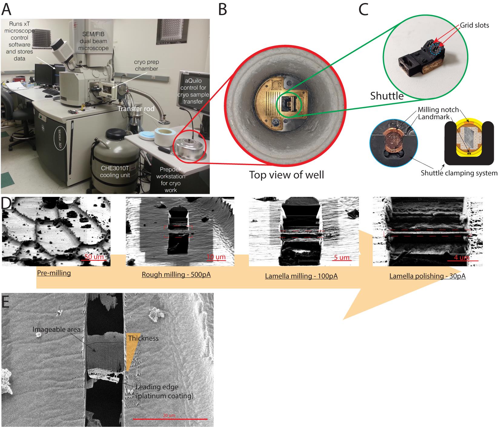
Figure 4. Loading of the clipped grids in the FIB/SEM with the Quorum PP3000T system. (A) Global view of the cryo-FIB/SEM setup. CHE3010T is the liquid nitrogen tank that cools down the flowing nitrogen, keeping the sample at cryogenic temperature. (B) Top view of the well where the grids are loaded in the shuttle. The shuttle is mounted on a hinge system and is seen vertical in this example. (C) Top: Picture of the shuttle that can fit two grids. Bottom: Top view of the grid loaded in the shuttle (left) and simplified diagram of the clamping system (right). Notice the milling notch and peel are facing upwards. This is crucial for successful milling. (D) FIB views of the milling process of a lamella in the periclinal cell wall. The lamella is boxed in orange. What is seen above and below the lamella is in the background. (E) SEM view of the final lamella shown in (D). Notice that the lamella is surrounded by dark holes above and below it. This ensures that the electron beam in the TEM will have a clear path through the lamella to the detector.Transfer grid boxes with clipped grids to the well.
Load the grids in the two slots (it is also possible to load the grids one by one to avoid too much in-chamber ice contamination during milling) and make sure milling notch is positioned vertically (see Note 4, Figure 4C). This will ensure that the peel is presented parallel to the FIB beam.
Pump down the well, load the shuttle on the transfer rod, and connect the rod to the cryo-preparation chamber.
Note: Cryogenic temperature during the transfer of the rod from the well to the preparation chamber is solely maintained by the vacuum. It is imperative to go as quickly as possible during this step to avoid devitrification.
Platinum sputter coat at 15 mA for 60 s.
Transfer the shuttle from the preparation chamber to the SEM chamber.
Screen the grid and identify areas of interest.
For each spot, save the x and y coordinates, proceed to setting the stage to eucentric height, and update their z coordinate (see Note 5).
For each spot, set up beam coincidence and update their z coordinate (see Note 5).
Optionally, if using the GIS needle for adding an extra coating layer of platinum, proceed as follows:
Go to a spot away from the loaded grids. For convenience, save the coordinates as “flush out spot” in order to call this position easily in the future.
Lock stage position.
Take a demagnified picture to make sure the stage is out of the field of view.
Insert GIS needle and open valves for approximately 15 s as a flush out step.
Take a picture to make sure needle is inserted.
Retract needle and unlock stage position.
Take a picture to make sure needle is retracted.
Recall milling position.
Set Z height to eucentric +2 mm.
Lock stage position.
Insert GIS needle and open valves for approximately 3–5 s.
Retract needle and take picture to make sure it retracted.
Unlock stage position.
Note: In between each milling step, astigmatism and focus must be checked away from the milling region.
Set stage angle as low as possible without hindering the field of view of the FIB beam (see Note 6).
Set the SEM imaging conditions to 5 kV and 27 pA in order to accurately assess lamella thickness.
Set beam intensity to 1 nA and milling pattern to “Clean Cross Section” (CCS) and select the “Si-ccs” application with a dwell time of 1 μs and a Z size between 1 and 3 μm (Figure 4D and Table 1), until the initial lamella is approximately 3 μm thick.
Set beam intensity to 0.5 nA (Figure 4D and Table 1).
Note: According to Schaffer et al. (2017), in order to have a homogenously thick lamella, the lamella has to be rocked back and forth when milling the underside and the topside, respectively.
Increase angle +1° and shave off approximately 1 μm of the top of the lamella (Table 1).
Increase angle -1° and shave off approximately 1 μm of the bottom of the lamella (Table 1). The lamella should be approximately 1 μm thick (Figure 4D).
Set beam intensity to 100 pA (Table 1).
Increase angle +0.5° and shave off approximately 200 nm of the top of the lamella (Table 1).
Increase angle -0.5° and shave off approximately 200 nm of the bottom of the lamella (Table 1). The lamella should be approximately 600 nm (Figure 4D).
Set beam intensity to 30 pA (Table 1).
Set the angle to the original milling angle and shave off the top of the lamella until it reaches its final thickness of approximately 200 nm (Figure 4D).
Optionally, to reach final thickness, beam intensity can be set to 10 pA.
Note: It is important to have set beam coincidence in order to be able to monitor lamella thickness, especially towards the final stages of milling where the lamella is getting thin and very fragile (see Note 7 for more details).
Iterate steps D12 to D23 for other milling targets on the grid.
When switching to other grid, set the stage angle to 0 and pan over to the other grid.
Note: For ease of navigation save left and right grid slot positions in order to easily recall these positions.
Iterate steps D8 to D23 for screening and milling the other grid.
When done screening both grids, set the stage angle to 0° and come back to loading position.
Note: For ease of navigation, loading position should also be saved for easy recall.
Close valves of the electron and FIB beam.
Fetch the shuttle with the transfer rod and transfer it to the cryo-preparation chamber.
Transfer back the shuttle into the precooled preparation well.
Secure the grids back into the grid box.
For loading and screening/milling new grids, iterate steps D4 to D31.
Cryo-ET screening and tilt series acquisition
Note: Only the key points of loading the grids for observing lamellae will be emphasized. In-depth information can be found online (https://em-learning.com/login/index.php). This run-through is relevant for the use of the Titan Krios cryo-TEM operated through SerialEM, a highly modular, scriptable software (Mastronarde, 2003). The steps detailed here to acquire the tilt series are meant for data acquisition on lamella as performed in Nicolas et al. (2022). For a more global understanding of what the different used options do and how this integrates in the spectrum of possible tomography workflows, please refer tohttps://bio3d.colorado.edu/SerialEM/hlp/html/main_index.htmand the SerialEM video serieshttps://www.youtube.com/playlist?list=PLGggUwWmzvs-DV4jCapSl5XQ-hpAXtzMb.
Precool the loading station and the NanoCab (Figure 5A, Video 3, steps 1 and 2).
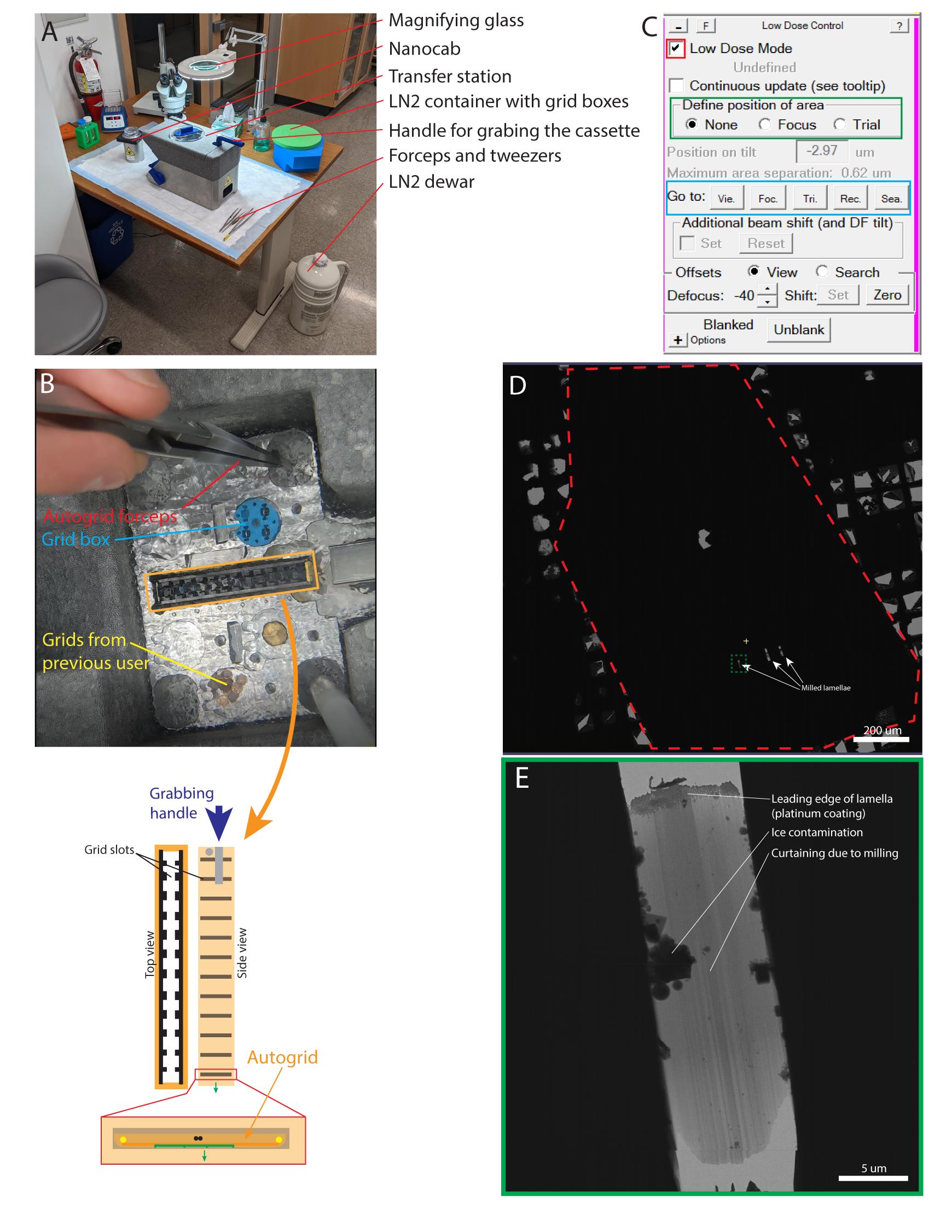
Figure 5. Loading the FIB milled grids in the Krios. (A) Global view of the loading station. (B) Top: Top view of the well of the loading station showing the autogrid forceps (red), open grid box containing three grids (blue), grids from the previous user (yellow), and the Krios cassette (orange outline). Bottom: Diagrams of the cassette from the top and side (left and right, respectively), with a magnified view of one grid slot to show the orientation of the grid in the cassette. Green arrow shows how the sample side of the autogrid should face towards the tip of the Krios cassette (as opposed to the side grabbed by the handle, blue arrow); the two dots are the two landmarks on the FIB autogrid indicating the axis of the notch. They should be positioned horizontally in the cassette. (C) Low dose control panel in SerialEM. Red square ticked indicates low dose mode is active. Green rectangle are the radio buttons to visualize the focus and trial spots. Blue rectangle allows to switch between the different imaging modes defined as “View,” “Focus,” “Trial,” “Record,” and “Search.” (D) Atlas montage of the whole grid. (E) View image (×2,250 magnification) of a lamella. See also Video 3. Video 3. Loading of the milled grids in the Krios.
Loading procedure is divided into five steps: i) cooling down of the loading station, ii) cooling down of the NanoCab, iii) transfer of the grid boxes in the loading station, iv) loading of the grids in the Krios cassette, and v) loading of the Krios cassette in the Titan Krios microscope. Note that the experimenter in this video is not wearing the recommended protective eyewear and insulating gloves.Transfer grid box with milled grids in transfer station (Video 3, step 3).
Put the grids in the slots of the cassette, so that the long axis of the lamellae is perpendicular to the tilt axis of the grid holder, leaving slot #1 free (commonly used slot for cross-grading grid) (see Note 8, Figure 5B, and Video 3, step 4).
Using the handle in the loading station, clamp the cassette and push it in the NanoCab (Video 3, step 4).
Transfer the NanoCab to the docking station of the microscope and load the cassette (Video 3, step 5).
When the cassette is loaded, let the cartridge gripper cool down to < -165° and start an inventory of the cassette.
Load a grid.
In the Low Dose panel, tick Low Dose Mode (Figure 5C, red square).
Generate a low magnification (search mode, x82) atlas of the grid to spot the lamellae (Figure 5D): Navigator > Open (will open a new Navigator panel); Navigator > Montage & Grids > Setup Full Montage (see Note 9); select the place holder of the file and the name of the atlas file.
Montage Controls > Start.
Spot good looking lamella: no hexagonal ice due to failed vitrification, no cubic ice due to devitrification, and electron-lucent (clear looking). Acquire a view image (×2,250) of the lamella (Figure 5E). Make sure the lamella appears vertical (perpendicular to the tilt axis).
Take a view image of the lamella and make sure it is centered.
Set the stage to eucentric height: Tasks > Eucentric – Rough. In the Navigator panel, select the object corresponding to the lamella and Update Z.
Note: Regularly save the navigator panel in case SerialEM crashes: Navigator > Save as…
Before going any further, go into an empty area near the lamella, Navigator panel > Add Stage Position to record this empty area for tuning the beam.
Go to the working magnification (record or preview), center/tune the energy filter, and perform a gain/dark reference in counting mode using Gatan DM3 software.
Tasks > Setup Autocenter… to set up the Autocenter beam function. Get out of low dose mode and follow instructions. Get back into low dose mode once this is set up. Now Tasks > Autocenter Beam will center the beam by focusing the beam and doing edge detection.
Define areas of interest where tilt series will be acquired by using the Anchor Maps function in the Navigator panel (see Note 10). If correctly done, the anchor maps should appear as blue outlines on the view image of the lamella.
Camera & script panel > view to have a global view of the lamella with acquisition areas (blue rectangles).
Navigator panel > select the first Sec 0 – AnchorHM.mrc item, tick Tilt series > Set tilt series acquisition parameters in the pop-up panel, and define tilt series parameters (see Note 11, Figure 6A, green rectangles for mandatory parameters and blue rectangles for optional control of dose spread along the tilt series).
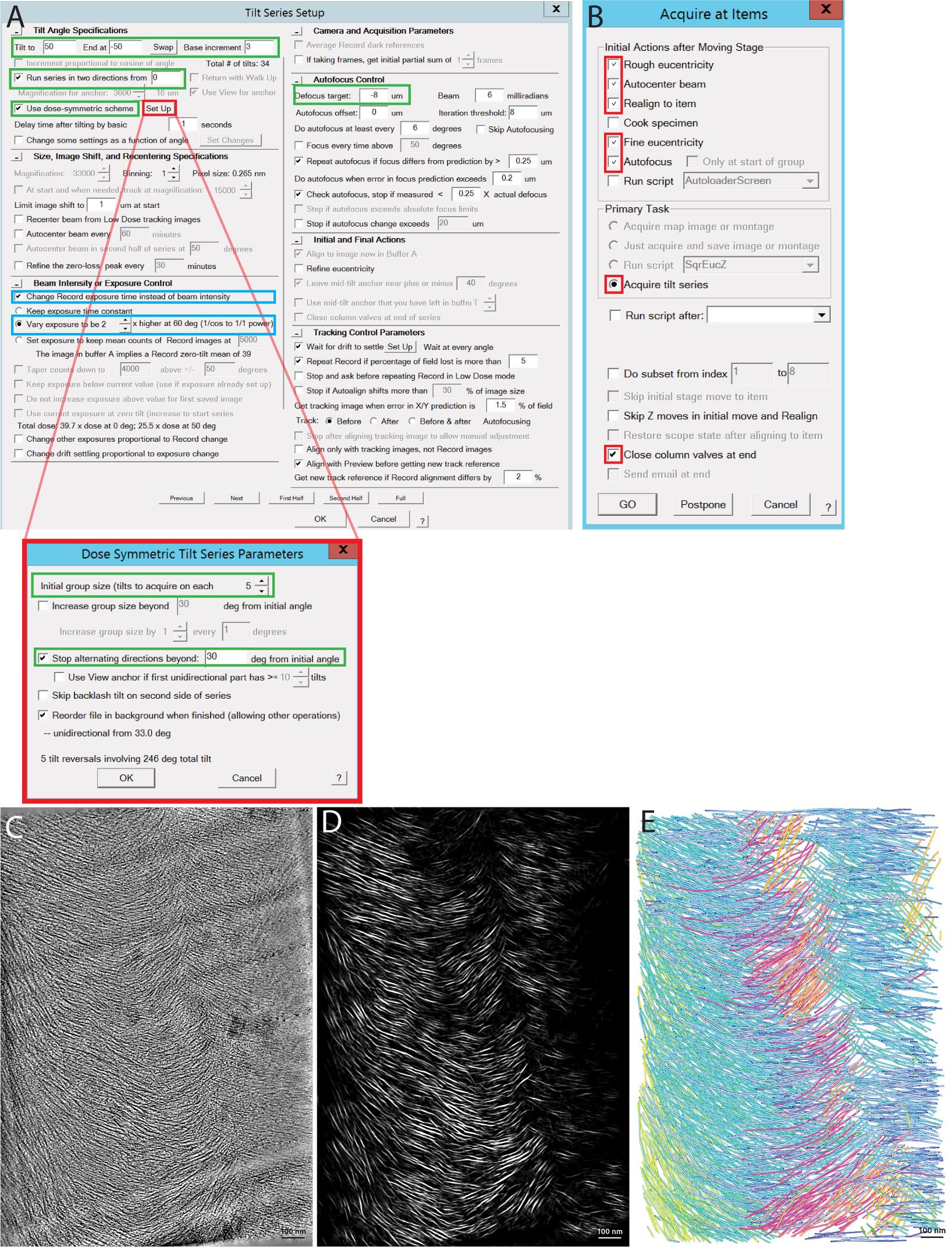
Figure 6. Setting up tilt series acquisition parameters. (A) Tilt series acquisition window. The green rectangles are the bare minimum parameters to be set up. In this example, a tilt series ±50° with a base increment of 3° using a dose symmetric scheme (see dose symmetric pop-up window in red and description below) with a target defocus of -8 μm. Optionally, the exposure can be set to vary according to tilt angle in order to distribute the dose optimally (blue rectangles). In the dose symmetric panel, at least two of the parameters need to be set (green rectangles). In this example, initial group size was set to 5 and alternation is set to end at 30°. This means that from 0 to ±30°, the stage will rock back and forth every five tilt images. After 30°, the stage will go linearly from ±30° to ±50°. (B) Acquire at items window. The typical checkboxes to activate are highlighted in red. This means that the stage will recall the position of the area to acquire, align it using the anchor maps as reference (realign to item), auto center the beam, do rough and fine eucentricity on the position, do autofocus, and start the tilt series. Valves will be closed when all tilt series are acquired. (C) Slice of a cryo-tomogram acquired on a cell wall lamella. The long rod-like densities are the cellulose fibers. (D) Slice of a probability map generated by the EMAN2 CNN trained to recognize the cellulose fibers on tomograms such as (C). (E) Template matching–based vector field generated by AMIRA from the CNN maps such as (D). These vector fields were used to extract per-fiber parameters used for analysis.Tick Edit focus and check whether the focus/trial spot is not overlapping with another tilt series to be acquired and that it is on the tilt axis.
Repeat steps E19 to E20 to set up remaining tilt series.
To edit the parameters of select tilt series, Navigator panel > TS Params.
When all tilt series are set up, Navigator > Acquire at items and tick Rough eucentricity, Fine eucentricity, Autocenter beam, Realign to item, and Autofocus; Acquire tilt series and tick Close column valves at end if needed (Figure 6B, red squares)
Reiterate steps E12 to E23 on the subsequent lamellae.
Data analysis
Note: Detailed description of tomogram reconstruction, CNN training, and fiber tracing exceeds the scope of this protocol paper, which focuses on the sample preparation and data acquisition. Instead, we invite the reader to visit the following pages for the different data analysis steps:
Tomogram reconstruction
For ETOMO reconstruction tutorial, please visit (https://bio3d.colorado.edu/imod/doc/patchTrackExample.html). An example of a reconstructed tomogram of the onion cell wall is shown in Figure 6C.
For ARETOMO automated alignment and reconstruction tutorial and manual, please visit https://drive.google.com/drive/folders/1Z7pKVEdgMoNaUmd_cOFhlt-QCcfcwF3 and refer to Zheng et al. (2022) (see Note 12). See also the following script for batch contrast transfer function correction and reconstruction using ETOMO and ARETOMO: http://dx.doi.org/10.13140/RG.2.2.31326.31043.
For EMAN2 automated alignment and reconstruction tutorial, please visit https://blake.bcm.edu/emanwiki/EMAN2/e2tomo (see Note 12).
CNN training and application
For training and application of CNNs with EMAN2, please visit https://blake.bcm.edu/emanwiki/EMAN2/Programs/tomoseg for a complete tutorial. An example of CNN segmented map of the onion cell wall is shown in Figure 6D.
Tracing of fibers with Amira – Xtracing plugin
For understanding the significance of the parameters used to trace the fibers, please refer to Rigort et al. (2012).
For a complete run-through to detect fibers in a tomogram, please refer to the Amira help documentation for the Xtracing extension. An example of a fiber-traced map of the onion cell wall is shown in Figure 6E.
Notes
White, fresh, and hard onions are preferrable. If possible, choosing big onions will allow for more material. In this study, the onions were usually bought the day prior to freezing and stored in the fridge. As effective peeling is not necessarily consistent between onions, it is therefore best to acquire a couple onions each time in case one is not peeling well.
EM grid boxes come in multiple shapes and forms. Classically they accommodate four grids. To avoid contamination, the best are the ones with a notched lid that allows opening one slot at a time (Mitegen #M-CEM-CGBSW1 and/or M-CEM-71166-10). Autogrid grid boxes number 1 through 4 are good for storing clipped grids (Mitegen M-CEM-7AGB).
Different types of grids were used. The goal in mind was to avoid accumulation of unblotted water underneath the peel, causing an increase of the total thickness of the sample to be milled and, in turn, hindering lamellae generation. Non-filmed grids (only copper grids) were tested. Despite giving extremely good blotting results, the cell wall is not supported by carbon, which caused instability during the final stages of milling, translated by a vibration of the final lamellae, impossible to thin down to final thickness. Quantifoil R17/5 (17 μm diameter holes spaced approximately 5 um) gave really good blotting results and lamella polishing stability. We therefore advise the use of Quantifoil R 17/5 grids (EMS # Q210CR175) or R 2/2, which is also a good compromise (EMS # Q250CR1).
Onion epidermal cells elongate in an anisotropic fashion, resulting in rectangular-like shapes. Having the peel presented to the FIB gun so that the long side of the rectangle-like cells is parallel to the FIB beam path allows more space for milling on the periclinal cell wall compared to when it is presented perpendicular to the FIB beam. The small rectangular-shaped cuts of cell wall (section B9 and 10) are dragged on the London Finder Quantifoil grid so that the long arrow (notch) on the grid is parallel to the long side of the rectangular peel (Figure 2C). Then, during the clipping stage, it is important to align the arrow on the Quantifoil grid with the notch of the autogrid (Figure 3).
Eucentric height is important in order to be able to tilt the stage without having significant x and y shift of the milling target. It can be first set by aiming at a contamination at the working magnification. Start at 0° and set the scan time to very fast. Increase the tilt angle by 5° increments until 20° and recenter the target for each increment using the Z slider. It is important to not shift in x and y during the procedure but just move the stage in z.
For further tuning, beam coincidence is established in order to have the milling target at the height where the SEM and FIB beam coincide. This is very useful for continuous monitoring with the SEM beam of the milling progress. To do so, center on a feature with SEM beam, image with the FIB beam, and center on the same feature by changing the Z-height of the sample (the offset should only be vertical). Then, recenter with SEM beam on feature using x and y shifts and repeat operation until the two images coincide on the same spot. Note that this needs to be done on each target.
After beam coincidence has been set, decrease the angle of the stage by 1° increments and check the FIB image. As long as the image is clear with no distortions or dark objects in the foreground, continue decreasing the angle. As soon as the bottom of the image suffers from distortions or a dark object is occluding the bottom of the image, the angle is too low. The last angle with a clear image is the shallowest angle usable for milling.
While some exclusively use the FIB view to monitor lamella thickness, SEM view informs on thickness homogeneity and overall shape and length on the lamella. It is important to monitor the thickness of the lamella using a combination of voltage and current that creates the smallest interaction volume possible. Around 5 kV – 27 pA is appropriate. At this setting, an approximately 200 nm thin lamella will appear homogenously black (Figure 4E). When this tint is reached, the lamella is considered ready for cryo-ET.
For on-lamella tilt series acquisition on a complete ±60° range, it is necessary to position the short side of the lamella parallel to the tilt axis of the goniometer in the microscope. In Thermo Fisher microscopes that are loaded with the standard grid cassette, this is done by positioning the FIB milling notch or the sputter-coating marks (only possible if the sample is sputter coated in PP3000T type shuttle), or the two black contiguous dots of the FIB autogrid sideways in the loading cassette (Figure 5B).
The magnifications used for this study are the following: ×82 (search mode), ×2,250 (view mode), and ×26,000 (record, preview, trial, and record modes).
To manage multiple magnifications, the Navigator > Imaging states can be used to store imaging states (magnification, illuminated area, 1st condenser lens parameters, etc.).
To modify on the fly an imaging mode:
Go into this imaging mode in the Low Dose Control panel > “Go to (view mode of choice).”
Camera&Script panel > click on the corresponding imaging mode to set the microscope accordingly and record an image > Low Dose Control panel > tick “continuous update” > modulate C2 with Intensity knob and check dose rate > untick "continuous update.”
To set up anchoring images, File > Open New and create two files, AnchorHM (for high magnification maps) and AnchorLM (for low magnification maps).
Go to the first area of interest (Navigator panel > Go to XY).
Buffer Control panel > Go through open files with “To file” to set the active file as AnchorHM (visible in the top window bar of SerialEM).
Camera&Script panel > Preview.
Buffer Control panel > “Save Active”.
Navigator panel > New map.
Buffer Control panel > “To file” to set the active file as AnchorLM.
Camera&Script panel > View.
Buffer Control panel > “Save Active”.
Navigator panel > New map.
Navigator panel > Tick “for anchor state”.
Go to second area of interest (Navigator panel > Go to XY).
Buffer Control panel > “To file” to set the active file as AnchorHM.
Acquisition panel > Preview.
Buffer Control panel > “Save Active”.
Navigator panel > New map.
Navigator panel > Anchor map. This will automatically set AnchorLM as active file. Take a View image, save it, and make a new anchor map.
Go to third area of interest (Navigator panel > Go to XY).
Make sure the active file is AnchorHM.
Camera&Script panel > Preview.
Navigator panel > Anchor map.
Repeat the last four bullet points for all the other areas of interest.
When setting up the tilt series acquisition parameters, the main goal is to expose the area of interest to the lower total dose possible, which damages the sample over time, but also to be in the optimal dose range for the detector in order to count electrons accurately (approximately 15 e-/px/s dose rate after the sample on a K3 detector in Correlated Double Sampling mode, CDS). For a tilt series acquired on an approximately 200 nm thick lamella, 80 e-/A2 total dose works well. To compute the total dose the sample will be exposed to, we use the following equation:

The before sample dose rate is measured by going to an empty area near the lamella and acquiring a Preview or Record image to read out the dose rate in e-/px/s.
Exposure time is set by going to Acquisition panel > Setup parameters > Exposure time. This parameter can be modified accordingly in order to lower the total dose.
Number (#) of exposures is defined by the tilting range and the tilt increment:
Tilting range is usually set to ±60° or ±50°.
Increment set to 3°.
Pixel size depends on the magnification. The smaller the pixel size (increased magnification), the higher the total dose will be.
The following Excel tool allows to conveniently calculate the total dose: DOI: 10.13140/RG.2.2.31306.85442.
For the tilt scheme, the associated study to this protocol used a bidirectional scheme starting from 0°. Nowadays, it is standard to acquire using a dose symmetric scheme (Figure 6A, red inset) in order to prioritize lower tilts before high resolution details are destroyed by the electron beam. The following default parameters for the dose symmetric scheme work well:Initial group size: 5.
Stop alternating directions beyond 30° from initial angle.
Reorder file in background when finished.
Recipes
HEPES buffer (HEPES 20 mM + Tween-20 0.1%, pH 6.8, 50 mL)
238 mg of HEPES powder
50 μL of Tween-20 100%
Quantity sufficient for 50 mL with DI water
pH 6.8 with KOH 1 M
This buffer can be prepared ahead of time and stored at room temperature. Make sure it is clear of precipitants before use.
CAPS buffer (50 mM, pH 10, 50 mL)
553 mg of CAPS powder
Quantity sufficient for 50 mL with DI water
pH 10 with NaOH 1 M
This buffer can be prepared ahead of time and stored at room temperature. Make sure it is clear of precipitants before use.
Pectate lyase at 4.7 U/mL (5 mL)
8 μL of the commercial solution (kept at 4 °C) in 5 mL of CAPS buffer 50 mM (see Recipe 2)
Incubate peels for three hours.
Enzymatic solution was always prepared fresh and kept on ice before use.
BAPTA 2 mM (50 mL)
48 mg of BAPTA powder
Quantity sufficient for 50 mL with DI water
This solution was always prepared fresh and could be kept at room temperature for the duration of the experiment.
Acknowledgments
The work related to this protocol was supported by the Howard Hughes Medical Institute (HHMI) and grant R35 GM122588 to Grant J Jensen, and Austrian Science Fund (FWF): P33367 to Florian KM Schur. Cryo-EM work was done in the Beckman Institute Resource Center for Transmission Electron Microscopy at Caltech.
This article is subject to HHMI’s Open Access to Publications policy. HHMI lab heads have previously granted a nonexclusive CC BY 4.0 license to the public and a sublicensable license to HHMI in their research articles. Pursuant to those licenses, the author-accepted manuscript of this article can be made freely available under a CC BY 4.0 license immediately upon publication.
Competing interests
There are no conflicts of interest or competing interests.
References
- Chen, M., Dai, W., Sun, S. Y., Jonasch, D., He, C. Y., Schmid, M. F., Chiu, W. and Ludtke, S. J. (2017). Convolutional neural networks for automated annotation of cellular cryo-electron tomograms. Nat Methods 14(10): 983-985.
- Dimchev, G., Amiri, B., Fassler, F., Falcke, M. and Schur, F. K. (2021). Computational toolbox for ultrastructural quantitative analysis of filament networks in cryo-ET data. J Struct Biol 213(4): 107808.
- Dubochet, J. (2007). The physics of rapid cooling and its implications for cryoimmobilization of cells. Methods Cell Biol 79: 7-21.
- Kafle, K., Xi, X., Lee, C. M., Tittmann, B. R., Cosgrove, D. J., Park, Y. B. and Kim, S. H. (2014). Cellulose microfibril orientation in onion (Allium cepa L.) epidermis studied by atomic force microscopy (AFM) and vibrational sum frequency generation (SFG) spectroscopy. Cellulose 21(2): 1075-1086.
- Kremer, J. R., Mastronarde, D. N. and McIntosh, J. R. (1996). Computer visualization of three-dimensional image data using IMOD. J Struct Biol 116(1): 71-76.
- Mastronarde, D. N. (1997). Dual-axis tomography: an approach with alignment methods that preserve resolution. J Struct Biol 120(3): 343-352.
- Mastronarde, D. N. (2003). SerialEM: A Program for Automated Tilt Series Acquisition on Tecnai Microscopes Using Prediction of Specimen Position. Microsc Microanal 9(S02): 1182-1183.
- Mastronarde, D. N. (2005). Automated electron microscope tomography using robust prediction of specimen movements. J Struct Biol 152(1): 36-51.
- Mastronarde, D. N. and Held, S. R. (2017). Automated tilt series alignment and tomographic reconstruction in IMOD. J Struct Biol 197(2): 102-113.
- Nicolas, W. J., Fassler, F., Dutka, P., Schur, F. K. M., Jensen, G. and Meyerowitz, E. (2022). Cryo-electron tomography of the onion cell wall shows bimodally oriented cellulose fibers and reticulated homogalacturonan networks. Curr Biol 32(11): 2375-2389 e2376.
- Rigort, A., Gunther, D., Hegerl, R., Baum, D., Weber, B., Prohaska, S., Medalia, O., Baumeister, W. and Hege, H. C. (2012). Automated segmentation of electron tomograms for a quantitative description of actin filament networks. J Struct Biol 177(1): 135-144.
- Schaffer, M., Engel, B. D., Laugks, T., Mahamid, J., Plitzko, J. M. and Baumeister, W. (2015). Cryo-focused Ion Beam Sample Preparation for Imaging Vitreous Cells by Cryo-electron Tomography. Bio-protocol 5(17): e1575.
- Schaffer, M., Mahamid, J., Engel, B. D., Laugks, T., Baumeister, W. and Plitzko, J. M. (2017). Optimized cryo-focused ion beam sample preparation aimed at in situ structural studies of membrane proteins. J Struct Biol 197(2): 73-82.
- Tang, G., Peng, L., Baldwin, P. R., Mann, D. S., Jiang, W., Rees, I. and Ludtke, S. J. (2007). EMAN2: an extensible image processing suite for electron microscopy. J Struct Biol 157(1): 38-46.
- Villa, E., Schaffer, M., Plitzko, J. M. and Baumeister, W. (2013). Opening windows into the cell: focused-ion-beam milling for cryo-electron tomography. Curr Opin Struct Biol 23(5): 771-777.
- Wagner, F. R., Watanabe, R., Schampers, R., Singh, D., Persoon, H., Schaffer, M., Fruhstorfer, P., Plitzko, J. and Villa, E. (2020). Preparing samples from whole cells using focused-ion-beam milling for cryo-electron tomography. Nat Protoc 15(6): 2041-2070.
- Zhang, T., Mahgsoudy-Louyeh, S., Tittmann, B. and Cosgrove, D. J. (2014). Visualization of the nanoscale pattern of recently-deposited cellulose microfibrils and matrix materials in never-dried primary walls of the onion epidermis. Cellulose 21(2): 853-862.
- Zhang, T., Vavylonis, D., Durachko, D. M. and Cosgrove, D. J. (2017). Nanoscale movements of cellulose microfibrils in primary cell walls. Nature Plants 3(5): 17056.
- Zhang, Y., Yu, J., Wang, X., Durachko, D. M., Zhang, S. and Cosgrove, D. J. (2021). Molecular insights into the complex mechanics of plant epidermal cell walls. Science 372(6543): 706-711.
- Zheng, S., Wolff, G., Greenan, G., Chen, Z., Faas, F. G. A., Bárcena, M., Koster, A. J., Cheng, Y. and Agard, D. (2022). AreTomo: An integrated software package for automated marker-free, motion-corrected cryo-electron tomographic alignment and reconstruction. bioRxiv: 2022.2002.2015.480593.
Article Information
Copyright
© 2022 The Authors; exclusive licensee Bio-protocol LLC.
How to cite
Nicolas, W. J., Jensen, G. J. and Meyerowitz, E. M. (2022). Focused Ion Beam Milling and Cryo-electron Tomography Methods to Study the Structure of the Primary Cell Wall in Allium cepa. Bio-protocol 12(23): e4559. DOI: 10.21769/BioProtoc.4559.
Category
Plant Science > Plant cell biology > Cell wall
Cell Biology > Cell imaging > Electron microscopy
Biophysics > Electron cryotomography
Do you have any questions about this protocol?
Post your question to gather feedback from the community. We will also invite the authors of this article to respond.