- Protocols

- Articles and Issues
- For Authors
- About
- Become a Reviewer

A Microfluidic Platform for Tracking Individual Cell Dynamics during an Unperturbed Nutrients Exhaustion
(*contributed equally to this work) Published: Vol 12, Iss 14, Jul 20, 2022 DOI: 10.21769/BioProtoc.4470 Views: 2933
Reviewed by: Zinan ZhouAlvaro BanderasDarrell Cockburn
Original research article
The authors used this protocol in:

Nov 2021
Advertisement


Protocol Collections
Comprehensive collections of detailed, peer-reviewed protocols focusing on specific topics


Abstract
Microorganisms have evolved adaptive strategies to respond to the autonomous degradation of their environment. Indeed, a growing culture progressively exhausts nutrients from its media and modifies its composition. Yet, how single cells react to these modifications remains difficult to study since it requires population-scale growth experiments to allow cell proliferation to have a collective impact on the environment, while monitoring the same individuals exposed to this environment for days. For this purpose, we have previously described an integrated microfluidic pipeline, based on continuous separation of the cells from the media and subsequent perfusion of the filtered media in an observation chamber containing isolated single cells. Here, we provide a detailed protocol to implement this methodology, including the setting up of the microfluidic system and the processing of timelapse images.
Keywords: Single-cell ecologyBackground
The proliferation capacity of microorganisms is tightly linked to the nature and availability of nutrients in their habitat. Exponential cell multiplication leads to the rapid exhaustion of resources, or to the secretion of metabolic byproducts in the medium, which can improve long-term population survival (Fabrizio and Longo, 2003; Enriquez-Hesles et al., 2021) or allow subsequent proliferation phases (Allen et al., 2006).
For instance, during its natural life cycle, budding yeast S. cerevisiae undergoes transitions between different metabolic phases due to the progressive consumption of nutrients in the environment. A rapid phase of sugar fermentation during which ethanol is produced is followed by a respiration phase where the cells consume the ethanol. In between these two phases, cells undergo a reversible proliferation arrest called the diauxic shift. Upon complete exhaustion of carbon sources, cells ultimately enter a dormant state, referred to as quiescence, a reversible proliferation arrest that lasts until new nutrient sources arise. Hence, S. cerevisiae’s fate is highly dynamic and tightly coupled to the continuous remodeling of its environment.
In addition, cells in this changing environment experience massive intracellular reorganizations in a very dynamic manner. Moreover, there is a high cell-to-cell variability in the cellular state reached by isogenic S. cerevisiae cells in a nutrient-deprived environment (Allen et al., 2006; De Virgilio, 2012; Sagot and Laporte, 2019). Lastly, the state of quiescence is sensitive to the nature of the nutrient deprivation (Klosinska et al., 2011), to the initial composition of the glucose medium (Fabrizio and Longo, 2003; Burtner et al., 2009; Smith et al., 2009), and also to the rate at which nutrients are consumed over time (Solopova et al., 2014). Therefore, studying quiescence at the population scale ignores cell-to-cell heterogeneities, while observing single cells responding to starvation with classical strategies such as microfluidics, is unable to consider the natural dynamics of a culture media (Li et al., 2013; Miles et al., 2021).
Studying the entry into quiescence requires longitudinal tracking of single cells while allowing cell proliferation to have a collective impact on the environment.
To this end, we have recently proposed a new microfluidic methodology to image single budding yeast cells during an unperturbed life cycle, from the fermentative phase to late quiescence, in an autonomously degrading environment (Jacquel et al., 2021). The cells trapped in an observation microfluidic device are constantly fed with the medium of a growing culture of cells, thus experiencing comparable environmental conditions.
In this protocol, we describe in detail how to run a typical experiment using this microfluidic system and provide a case study with a fluorescence single-cell pH cytosolic sensor during an unperturbed life cycle.
Materials and Reagents
Glass coverslips 0.15 mm in thickness, 24 × 50 mm (e.g., Knittel Glass)
Glass slide, any thickness >0.5 mm, 24 × 75 mm (e.g., Knittel Glass)
Plastic weighing boat
Razor blade (e.g., Swan Morton with n°10 blade)
1 mm biopsy punch (e.g., Kai medical)
Cutting mat (e.g., QIAGEN WB100020, FisherScientific, catalog number: 11323365)
Aluminum foil
Ethanol 70% and 100%
Clear removable tap (e.g., 3M magic tape)
“Spiral”, “Dust filter”, and observation microfluidic molds (see Figure 1). Designs available at https://github.com/TAspert/Continuous_filtration and (Goulev et al., 2017); can be produced by a standard photolithographic process (see details at Jacquel et al., 2021) or sent on demand.
1 m of 1 mm outer diameter Polytetrafluoroethylene (PTFE) tubes (e.g., Adtech Polymer Engineering 1.07 mm outer diameter, Fisher Scientific, catalog number: 11929445)
5 mL Syringe (e.g., Terumo)
23G needles (e.g., Terumo)
Budding yeast strain
Culture media (e.g., Yeast Extract Peptone supplemented with Dextrose, YPD)
Polydimethylsiloxane (PDMS) and cross-linking agent (Sylgard 184 from Dow Chemical) (see Recipes for preparation)
Equipment
Plasma cleaner (e.g., Diener, model: Zepto)
Peristaltic pump (e.g., Ismatec, model: IPC) or any other pump able to generate flow rates between 10 and 100 µL/min
Inverted epifluorescence microscope (e.g., Nikon, model: Ti Eclipse 2)
Oven (heating at 60°C)
Tweezers (e.g., Fine Science Tools, catalog number: 91100-16)
1 Erlenmeyer flask per condition (25 mL)
Vacuum desiccator (e.g., Nalgene, Thermo Fisher, catalog number: 5305-0609)
Vacuum pump (e.g., Millivac-Maxi Vacuum Pump, Merck, catalog number: SD1P014M04)
Orbital shaker (e.g., Solaris 2000, ThermoFischer, catalog number:SK2000)
For pHluorin observation:
Fluorescence emission source of peak excitation wavelengths at 390/18 and 475/28 nm (e.g., Lumencor, model Retra)
Filter cubes for peak excitation wavelengths at 390/18 and 475/28 nm, and collection at 525/50 nm (for both excitation wavelengths) (e.g., Chroma)
Software
To drive the microscope: Micromanager 2.0.0 (https://micro-manager.org) (Edelstein et al., 2014)
For image and data analysis: Matlab, including Matlab Toolbox “Image processing”, “Statistical analysis”, “Signal processing”, and the Matlab modules Phylocell + Autotrack (Goulev et al., 2017), https://github.com/gcharvin/phyloCell, https://github.com/gcharvin/autotrack or DetecDiv (Aspert et al., 2022).
Procedure
The whole protocol describes how to run an experiment with one condition. Details are given at specific points for running multiple conditions in parallel. This procedure works with haploid budding yeast cells but can be adapted by tweaking the dimensions of the devices in order to fit with similar cells.
Fabrication of the microfluidic devices (day -1)
Prepare the PDMS (cf. Recipe section). One spiral (5 g of PDMS required) and one dust filter (5 g required) are required per condition; the observation device can take up to 16 conditions (10 g required) (for description of molds, see Figure 1). Therefore, one condition requires approximately 20 g of PDMS, and an additional 10 g is required per additional condition.
Pour the PDMS into the three microfluidic molds and leave them at room temperature for ~5 min to let any potential bubbles leave the PDMS.
Bake the molds at 60–80°C for a few hours (at least 5 h at 60°C, or at least 2 h at 80°C) in an oven. Molds can be left overnight or over the weekend in the oven without a problem.
Carefully peel the chips off the molds using a razor blade, and cut exceeding sides on the cutting mat.
Turn the chip features up and punch holes using the 1 mm biopsy tool at the inlets of the PDMS devices. Four holes have to be punched on the observation device (per condition), three on the spiral, and two on the dust filter (Figure 1). Perform this operation on the cutting mat to not damage your tool.
Preparation of the devices (day 0)
Take the previously fabricated PDMS devices (cf part A), and carefully clean their surfaces using the cleaning tape.
Prepare one glass coverslip for the observation device and one glass slide per condition.
Put the chips in the chamber of the plasma cleaner, face-up, as well as the glass coverslip and slide(s). Close the chamber.
Vacuum the chamber to approximately 0.2 mbar. Then, inject dioxygen (or air) into it until a pressure of 0.7 mbar is reached (parameters may vary depending on the plasma cleaner).
Set the power to 10% and the timer to 20s, and generate the plasma (parameters may vary depending on the plasma cleaner).
Once the plasma exposure is done, take back the chips and glass cover from the chamber, and seal the chips to their respective glass cover. The spiral and dust filter can be put on the same glass slide for convenience. Do not press the chips too much against the glass (especially for the observation device) as it could collapse the chambers.
Put the assembled devices in a 60°C oven for 20min.
The chips are ready to be primed and loaded. This should be done no later than an hour after the plasma activation to keep the surfaces hydrophilic, to avoid the formation of air bubbles once the channels are filled with media.
Preparation of the cell culture (days -2, -1, and 0)
General note for the two following sections (C and D): All the media manipulations must be done under a sterile hood or close to a flame to prevent contaminations from other microorganisms. Antibiotics can be added to the medium to limit the probability of microbial contamination.
Thaw cells from -70°C on an agar plate and let them at 30°C for 2 or 3 days.
The day before the experiment, inoculate the cells in a culture tube of the same media as the experiment and let the cells grow overnight at 30°C with continuous shaking.
Note: All media used within the following steps need to be recently filtered to avoid dust particles and media crystals.
On the day of the experiment, prepare 25 mL of filtered liquid medium (typically, YPD) into a 50 mL Erlenmeyer, and resuspend cells to low OD (between 0.05 and 0.1). Put a sterile aluminum foil on the top of the Erlenmeyer to prevent microbial contamination while allowing air exchange between the room and the Erlenmeyer. Let the cells grow at room temperature with continuous shaking.
One to two hours before the desired start point of the time-lapse (see Note for details), load ~5 mL of the culture into a 5mL syringe, using a 23 G needle. This syringe will be used to load the microfluidic chambers. Put back the Erlenmeyer flasks containing the rest of the culture (~20 mL) under continuous shaking, during the preparation and the loading of the microfluidic device.
Note: The time at which cells are loaded within the device depends on the growth phase of the yeast life cycle to study. Example: To image the transition from fermentative growth to the diauxic shift, it is recommended to start cell loading 5 h before the end of the fermentative phase (i.e., 5h before the diauxic shift); 1 to 2 h are needed from the cell loading (step B6) to the beginning of the time-lapse, depending on the experimenter.
Priming and loading the microfluidic chip (day 0)
Clean and sterilize the PTFE tubes by running ethanol 70% and then air into them.
Connect the PTFE tubes as described in Figure 1, i.e., per condition, plug:
1) One tube from the pump to the dust filter
2) One tube from the dust filter to the inlet of the spiral (centered hole)
3) One tube from the external outlet of the spiral to the observation device
4) One tube from the internal outlet of the spiral to nothing
5) One tube from the outlet of the observation device to nothing
6) One tube from each of the two cell-inlets of the observation device to nothing
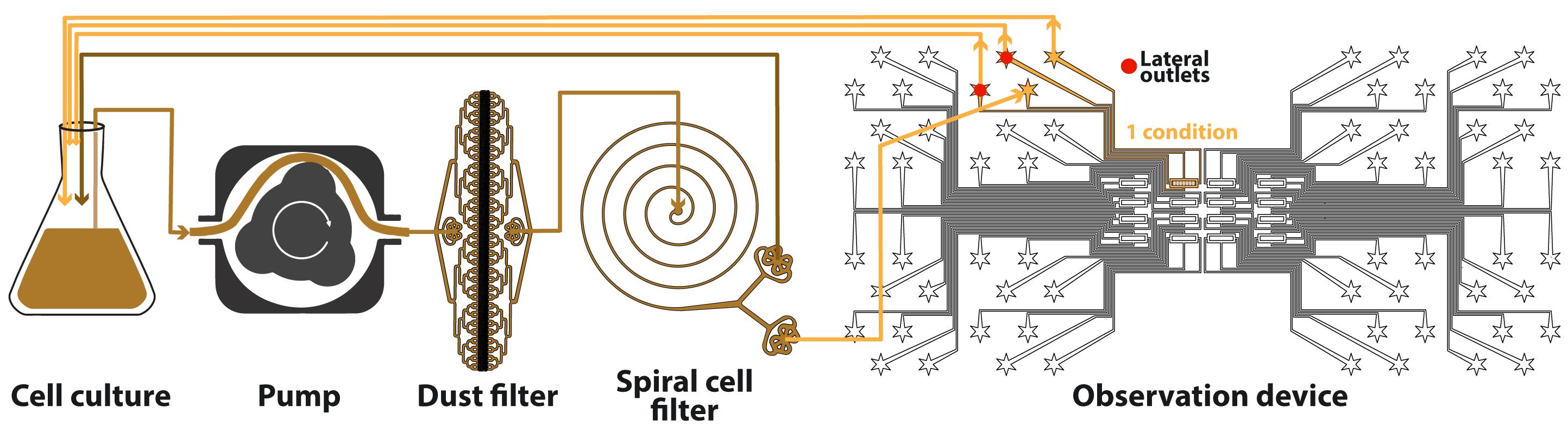
Figure 1. Schematic of the fluidic system. Colored lines represent tubes; the color indicates the concentration in cells (darker means higher). Arrows indicate flow direction at steady-state. The observation device contains 16 independent conditions, only one being used here.Once the cell culture is at the desired growth stage, remove it from the shaker.
Wipe the other end of the pump tube with a tissue and ethanol 100%, let it dry for a few seconds, and plug it into the Erlenmeyer through the aluminum foil. This inlet has to be in contact with the culture medium since it has to aspirate the culture medium into the pump and the whole microfluidic system. Seal the hole made into the aluminum using paper tape, to maintain sterility.
Switch the pump on with a flow rate of 50–100µL/min to prime the microfluidic system. The four tube ends of this system (the outlet of the spiral, two cell-inlets of the observation device, and the outlet tube of the observation device) can be momentarily put into an empty beaker (Figure 2, left). Let the medium flow for a few minutes to remove all the air from the fluidic system.
Figure 2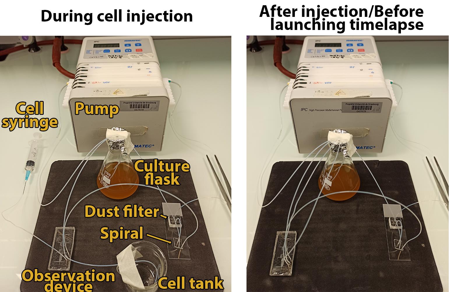
Figure 2. Picture of the fluidic system during (left) and after (right) the cell injection step.Wipe the outlet tube from the observation device with a tissue and ethanol 100%, let it dry for a few seconds, and plug it into the Erlenmeyer through the aluminum foil. This tube does not need to be in contact with the culture medium. At this time, only two tubes, the lateral tubes from the observation device, should remain unplugged.
Stop the pump. Take the syringe prepared in step C4 and connect it (via a 23 G needle) to one of the two lateral tubes (it does not matter which one) (Figure 2, left). Gently inject cells within the microfluidics device. It is recommended to check cell injection in real-time with a bench microscope to adjust the number of cells within microfluidics sub-chambers. The number of initial cells must be adjusted depending on the life-cycle phase of interest. To study cells from fermentation to quiescence, it is recommended to start with approximately 3–10 cells per chamber (Figure 3).
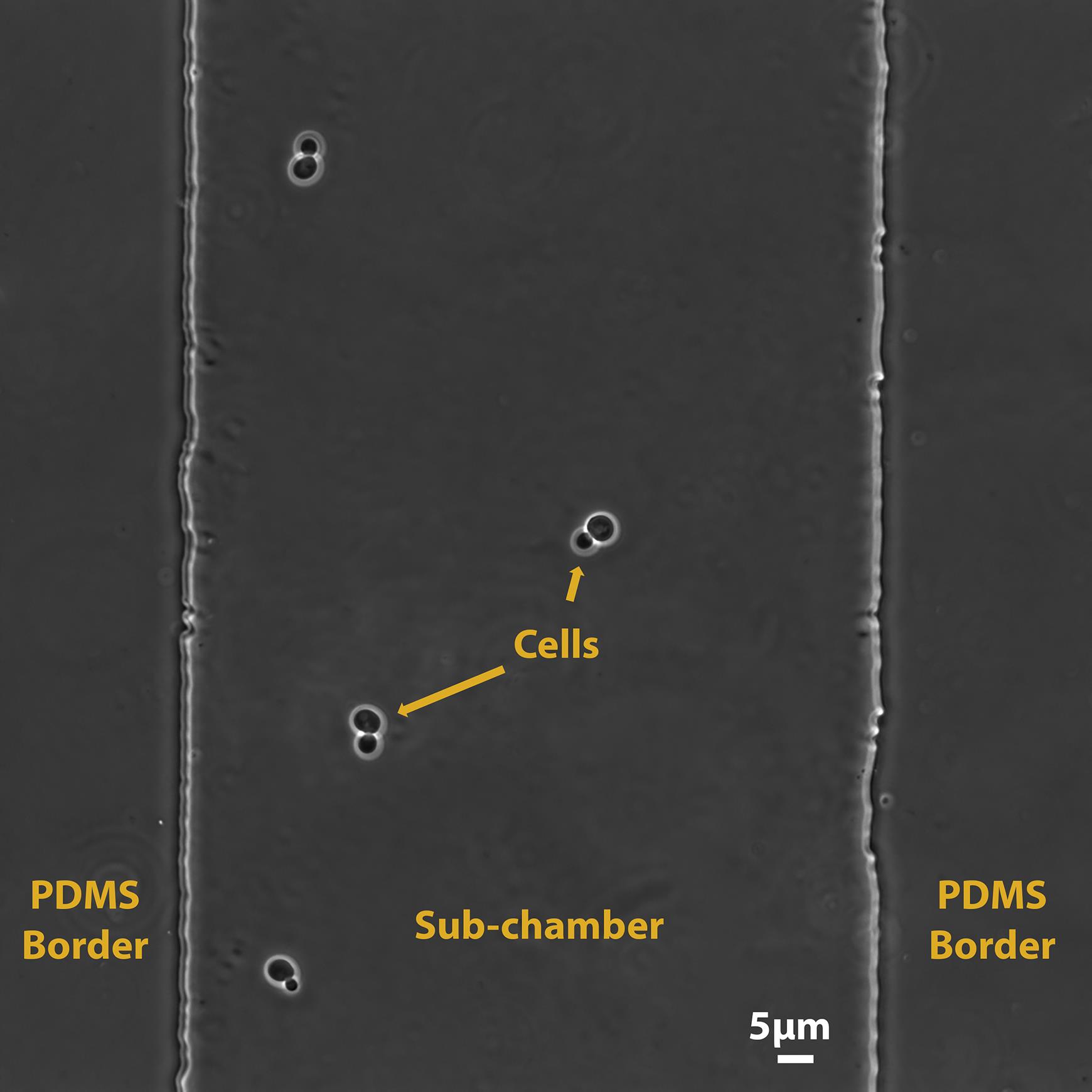
Figure 3. Typical field of view of a chamber of the observation device after cell injection.Disconnect the syringe from the PTFE tube. Wipe the lateral tubes with a tissue and ethanol 100%, let them dry for a few seconds, and plug them into the Erlenmeyer through the aluminum foil. At this time, the fluidic system should be in a closed loop (Figure 2, right).
Set up and start of the timelapse (day 0)
Bring the fluidic system (devices, tubes, Erlenmeyer, and pump) close to the microscope.
Install the observation device onto the sample holder of the microscope.
Place the Erlenmeyer onto an orbital shaker and the rest of the devices in a relevant place. The tubes can be secured using paper tape.
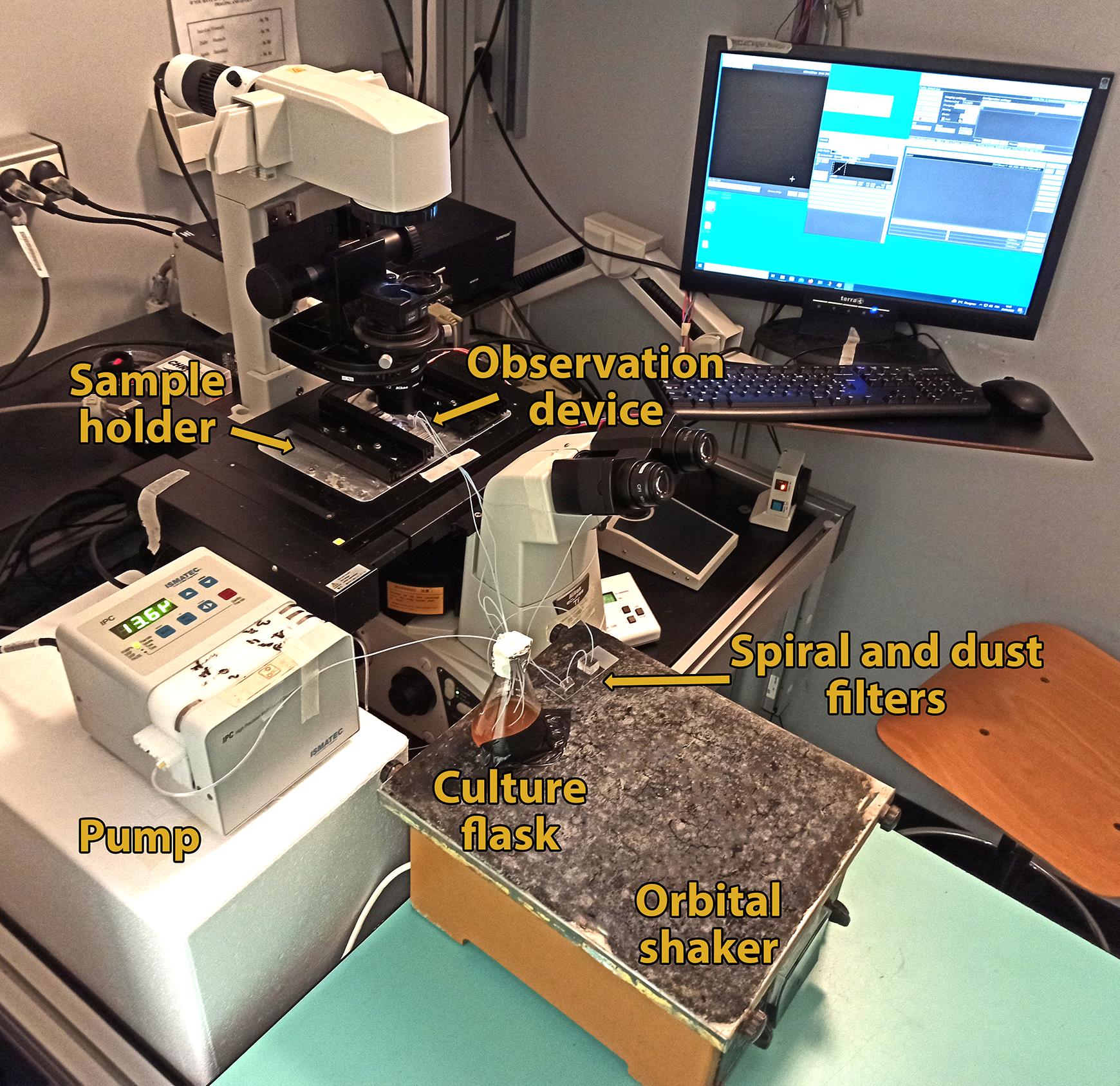
Figure 4. Picture of a typical fluidic and microscopy setup during the timelapse experiment.Switch the pump back on and set it to a flow rate of 80-120 µL/min (flow rate for optimal spiral filtration). The setup should be similar to the one in Figure 4.
Check that the media is properly flowing in all the tubes by checking for droplets at the outlets. If not, check for potential bubbles all along the tubes.
Set up the positions for the timelapse (typical position displayed in Figure 3), as well as the imaging conditions (channels, exposure, etc.). This can be done using Micromanager or any microscope controlling software. To image the pHluorin sensor, the fluorescence is acquired at two different excitation wavelengths (Peak excitation wavelengths at 390/18 and 475/28 nm) and collected for both excitation wavelengths at 525/50 nm (emission wavelength). Adjust excitation and emission wavelengths depending on the fluorescent protein.
Monitor the experiment throughout the days. In particular, check for potential leaking or clogging of the devices (notably from the dust filter device, which serves as a fluidic fuse), for potential loss of focus from the microscope, or potential contamination in the chamber.
Data analysis
As a case study, a data analysis workflow is described below, using the single-cell analysis of cytosolic pH using the ratiometric fluorescent sensor pHluorin (Mouton et al., 2020; Jacquel et al., 2021) as an example. This processing can be done in multiple ways using different software tools. Here, we use the custom Matlab addons Phylocell and Autotrack (https://github.com/gcharvin/phyloCell, https://github.com/gcharvin/autotrack). Tutorials for these software tools are available in their respective folders.
At the end of the timelapse experiment, load the data into PhyloCell.
Visualize the images series, and check that the cells grew following the expected different growth phases and that no apparent problem has occurred (contamination, loss of focus, air bubbles…).
Segment and track cells using the automatic batch segmentation workflow from Autotrack. Segmentation and cell tracking can then be corrected manually using PhyloCell if needed. Although segmentation is usually robust, a few tracking errors might require manual correction.
Note: Cell segmentation means determining cell contours on an image. Cell tracking means attributing a cell contour to a cell throughout the timepoints (to recapitulate the whole “life trajectory”.)
Once cells are correctly segmented and tracked, it is possible to measure the fluorescence of each cell segmented area, for each excitation wavelength, and for each timepoint. Subtract the background value from each wavelength (estimated from an area on the image depleted of cells).
Calculate the fluorescence ratio I390/I475, and convert it into pH using the pH calibration, for each timepoint. You now have access to the cytosolic pH of each cell throughout the timepoints.
Notes:
The pHluorin probe works as a ratiometric fluorescent cytosolic pH sensor. Depending on the cytosolic pH, the intensity of the light collected at the two different excitation wavelengths is modified, resulting in a modification of the light intensity ratio. To transform the fluorescence ratio into an absolute cytosolic pH value, a calibration must be done using the same system as the experiment [See supplementary section of Mouton et al. (2020); Jacquel et al. (2021) for details].
The fluorescent ratio within the vacuole is slightly different from the rest of the cytosol. However, excluding the vacuole from the analysis does not dramatically change the estimated value of the cytosolic pH.
Recipes
PDMS
Pour approximately 30 g of PDMS into a plastic weighing boat (for one condition).
Add curing agent in a 1:10 proportion (3 g in this case).
Thoroughly mix (for example, using a bent 1 mL tip) and degas the solution under a vacuum desiccator for approximately 30 min.
Acknowledgments
This work was supported by the Fondation pour la Recherche Médicale (FRM, B.J, and G.C.), the Agence Nationale pour la Recherche (T.A. and G.C.), the grant ANR-10-LABX-0030-INRT, a French State fund managed by the Agence Nationale de la Recherche under the frame program Investissements d'Avenir ANR-10-IDEX-0002-02.
This protocol is a related to our previous study published in eLife [Jacquel et al. (2021)], doi: 10.7554/eLife.73186.)
Competing interests
The authors declare no competing interests.
References
- Allen, C., Buttner, S., Aragon, A. D., Thomas, J. A., Meirelles, O., Jaetao, J. E., Benn, D., Ruby, S. W., Veenhuis, M., Madeo, F., et al. (2006). Isolation of quiescent and nonquiescent cells from yeast stationary-phase cultures. J Cell Biol 174(1): 89-100.
- Aspert, T., Hentsch, D. and Charvin, G. (2022). DetecDiv, a deep-learning platform for automated cell division tracking and replicative lifespan analysis. bioRxiv: 2021.2010.2005.463175.
- Burtner, C. R., Murakami, C. J., Kennedy, B. K. and Kaeberlein, M. (2009). A molecular mechanism of chronological aging in yeast. Cell Cycle 8(8): 1256-1270.
- De Virgilio, C. (2012). The essence of yeast quiescence. FEMS Microbiol Rev 36(2): 306-339.
- Edelstein, A. D., Tsuchida, M. A., Amodaj, N., Pinkard, H., Vale, R. D. and Stuurman, N. (2014). Advanced methods of microscope control using muManager software. J Biol Methods 1(2).
- Enriquez-Hesles, E., Smith, D. L., Jr., Maqani, N., Wierman, M. B., Sutcliffe, M. D., Fine, R. D., Kalita, A., Santos, S. M., Muehlbauer, M. J., Bain, J. R., et al. (2021). A cell-nonautonomous mechanism of yeast chronological aging regulated by caloric restriction and one-carbon metabolism. J Biol Chem 296: 100125.
- Fabrizio, P. and Longo, V. D. (2003). The chronological life span of Saccharomyces cerevisiae. Aging Cell 2(2): 73-81.
- Goulev, Y., Morlot, S., Matifas, A., Huang, B., Molin, M., Toledano, M. B. and Charvin, G. (2017). Nonlinear feedback drives homeostatic plasticity in H2O2 stress response. Elife 6: e23971.
- Jacquel, B., Aspert, T., Laporte, D., Sagot, I. and Charvin, G. (2021). Monitoring single-cell dynamics of entry into quiescence during an unperturbed life cycle. Elife 10:e73186
- Klosinska, M. M., Crutchfield, C. A., Bradley, P. H., Rabinowitz, J. D. and Broach, J. R. (2011). Yeast cells can access distinct quiescent states. Genes Dev 25(4): 336-349.
- Li, L., Miles, S., Melville, Z., Prasad, A., Bradley, G. and Breeden, L. L. (2013). Key events during the transition from rapid growth to quiescence in budding yeast require posttranscriptional regulators. Mol Biol Cell 24(23): 3697-3709.
- Miles, S., Bradley, G. T. and Breeden, L. L. (2021). The budding yeast transition to quiescence. Yeast 38(1): 30-38.
- Mouton, S. N., Thaller, D. J., Crane, M. M., Rempel, I. L., Terpstra, O. T., Steen, A., Kaeberlein, M., Lusk, C. P., Boersma, A. J. and Veenhoff, L. M. (2020). A physicochemical perspective of aging from single-cell analysis of pH, macromolecular and organellar crowding in yeast. Elife 9: e54707.
- Sagot, I. and Laporte, D. (2019). The cell biology of quiescent yeast - a diversity of individual scenarios. J Cell Sci 132(1): jcs213025.
- Smith, D. L., Jr., Li, C., Matecic, M., Maqani, N., Bryk, M. and Smith, J. S. (2009). Calorie restriction effects on silencing and recombination at the yeast rDNA. Aging Cell 8(6): 633-642.
- Solopova, A., van Gestel, J., Weissing, F. J., Bachmann, H., Teusink, B., Kok, J. and Kuipers, O. P. (2014). Bet-hedging during bacterial diauxic shift. Proc Natl Acad Sci U S A 111(20): 7427-7432.
Article Information
Copyright
![]() Aspert et al. This article is distributed under the terms of the Creative Commons Attribution License (CC BY 4.0).
Aspert et al. This article is distributed under the terms of the Creative Commons Attribution License (CC BY 4.0).
How to cite
Readers should cite both the Bio-protocol article and the original research article where this protocol was used:
- Aspert, T., Jacquel, B. and charvin, G. (2022). A Microfluidic Platform for Tracking Individual Cell Dynamics during an Unperturbed Nutrients Exhaustion. Bio-protocol 12(14): e4470. DOI: 10.21769/BioProtoc.4470.
- Jacquel, B., Aspert, T., Laporte, D., Sagot, I. and Charvin, G. (2021). Monitoring single-cell dynamics of entry into quiescence during an unperturbed life cycle. Elife 10:e73186
Category
Microbiology > Microbial cell biology > Cell isolation and culture
Environmental science
Cell Biology > Cell imaging
Do you have any questions about this protocol?
Post your question to gather feedback from the community. We will also invite the authors of this article to respond.