
- Submit a Protocol
- Receive Our Alerts
- EN

- Protocols

- Articles and Issues
- For Authors
- About
- Become a Reviewer

A Semi-throughput Procedure for Assaying Plant NADP-malate Dehydrogenase Activity Using a Plate Reader
Published: Vol 13, Iss 16, Aug 20, 2023 DOI: 10.21769/BioProtoc.4769 Views: 825
Reviewed by: Anonymous reviewer(s)
Original research article
The authors used this protocol in:
Aug 2022

Protocol Collections
Comprehensive collections of detailed, peer-reviewed protocols focusing on specific topics


Abstract
Chloroplast NADP-dependent malate dehydrogenase (NADP-MDH) is a redox regulated enzyme playing an important role in plant redox homeostasis. Leaf NADP-MDH activation level is considered a proxy for the chloroplast redox status. NADP-MDH enzyme activity is commonly assayed spectrophotometrically by following oxaloacetate-dependent NADPH oxidation at 340 nm. We have developed a plate-adapted protocol to monitor NADP-MDH activity allowing faster data production and lower reagent consumption compared to the classic cuvette format of a spectrophotometer. We provide a detailed procedure to assay NADP-MDH activity and measure the enzyme activation state in purified protein preparations or in leaf extracts. This protocol is provided together with a semi-automatized data analysis procedure using an R script.
Keywords: NADP-malate dehydrogenaseBackground
Chloroplast NADP-dependent malate dehydrogenase (NADP-MDH) catalyzes the reduction of oxaloacetate to malate using NADPH. To be active, this enzyme needs to be reduced by thioredoxins (TRX), ubiquitous thiol-disulfide oxidoreductases (Issakidis et al., 1994; Collin et al., 2003). In C3 plants, NADP-MDH is involved in the export of reducing power from the chloroplast to the cytosol via the malate valve (Scheibe, 2004). TRX-dependent activation of NADP-MDH makes the link between the chloroplast electron transport chain, the redox state of the chloroplast, and the other cell compartments (Scheibe and Dietz, 2012; Heyno et al., 2014). Hence, the redox state of NADP-MDH is considered as a proxy for the plant leaf cellular redox state. NADP-MDH redox state in protein preparations or in plant extracts is deduced from the ratio between initial/extractable (i.e., activity of the enzyme or extract, without pre-treatment) and maximal activity/enzyme capacity (i.e., activity of the enzyme or in the extract, after reductive activation by TRX) (Issakidis et al., 1994; Keryer et al., 2004).
NADP-MDH activity can be easily assayed spectrophotometrically by monitoring oxaloacetate-dependent NADPH oxidation at 340 nm (Jacquot et al., 1995). Here, we developed a plate-adapted protocol to assay NADP-MDH activity of a large number of samples at the same time, associated with a semi-automatized data analysis procedure using a user-friendly R script. Compared with the classic method in a 1 mL spectrophotometer cuvette, the plate format allows increasing the experimental replicates and/or tested samples or conditions, for a gain of time (estimated divided by three), and in data precision and reliability, at a lower cost (divided by five). We implemented this method to measure NADP-MDH activity in Arabidopsis leaf protein extracts and using purified preparations of recombinant sorghum NADP-MDH. Our method is applicable to measure the activity of virtually any plant species.
Materials and reagents
General materials and reagents
Oxaloacetic acid (OAA) (Sigma-Aldrich, catalog number: O-4126)
β-Nicotinamide adenine dinucleotide 2’-phosphate reduced (NADPH) (Roth, catalog number: AE14.3)
Dithiothreitol (DTT) (Sigma-Aldrich, catalog number: D9779)
Tris pH 7.9
Classic PCR plate 96 wells (Thermo Fisher Scientific, catalog number: AB0700)
Plate 96 wells (Genetix X6011 96well)
Recombinant TRX m type (stored at -20 °C) (Collin et al., 2003)
Materials and reagents specific for in vitro assay
Recombinant NADP-MDH (stored at -20 °C) (Issakidis et al., 1994)
Materials and reagents specific for ex planta assay
4–5-week-old Arabidopsis plants
Metallic beads (3 mm diameter)
Protease inhibitor cocktail for plant (Sigma-Aldrich, catalog number: P9599)
Tris pH 6.8
QubitTM Protein and Protein Broad Range (BR) Assay kits (Thermo Fisher Scientific, catalog number: Q33212)
Solutions
Extraction buffer for ex planta assay (see Recipes)
Activation medium for ex planta assay (see Recipes)
Activation medium for the in vitro assay (see Recipes)
Reaction medium (see Recipes)
Equipment
Tecan infinite m200 PRO plate reader (Tecan) with a 230–1,000 nm wavelength range
Multichannel pipettes, 12 channels able to pipette 2–50 μL (Eppendorf)
General-purpose tweezers (Fisher Scientific, catalog number: 17-467-231)
Thermal cycler for incubation (Applied Biosystems 2720 Thermal Cycler)
Qubit 2.0 fluorometer (Thermo Fisher Scientific, Q32866) (for ex planta assay) (see Note 1)
Refrigerated microcentrifuge (Thermo Scientific, catalog number: 75-772-441)
Tissue Lyser II bead mill (Qiagen, catalog number: 85300)
Software
R (https://www.r-project.org/) version 3.6.3 or later
RStudio (https://www.rstudio.com/) version 2022.07.1+554 or later
Excel (Microsoft)
Notepad++ (https://notepad-plus-plus.org/) or any software to read text files
Magellan version 7.2 (https://lifesciences.tecan.com/software-magellan)
Procedure
An overview of the procedure and data analysis workflow is presented in Figure 1.
For NADP-MDH ex planta activity, follow sections A and C. For recombinant NADP-MDH activity (in vitro) assay, follow sections B and C. As a general advice, because this protocol uses plates and can measure up to 12 samples at the same time, triplicate assays can be easily performed in parallel for each sample type and for each experimental condition (initial or maximal activity for ex planta activity, activation kinetics for recombinant enzyme).
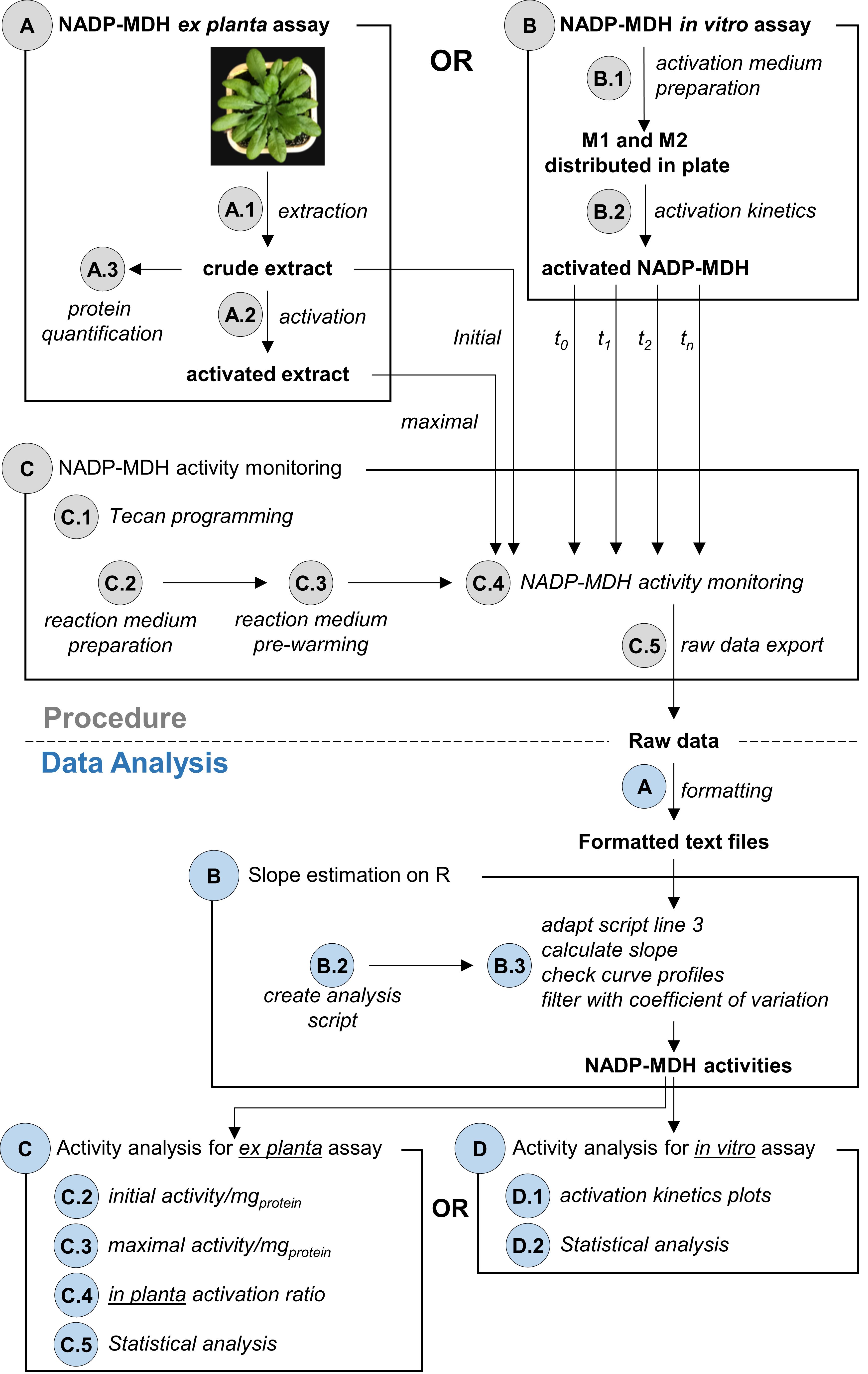
Figure 1. Overview of the procedure and data analysis workflow. Grey circles refer to corresponding procedure sections. Blue circles refer to corresponding data analysis sections. For NADP-MDH ex planta activity, follow procedures A and C and then analysis A, B and C. For NADP-MDH in vitro assay, follow procedures B and C and then analysis A, B and D.
Arabidopsis NADP-MDH extraction and activation, ex planta assay (alternative for B)
Extraction from leaf samples:
Using tweezers, collect one young adult leaf from a 4–5-week-old Arabidopsis plant in a collecting tube containing two metallic beads. Flash freeze samples in liquid nitrogen (see Note 2).
Grind sample in collecting tube by shaking using a bead mill (1 min at a frequency of 30 vibrations per second). Bead mill racks must be pre-chilled in liquid nitrogen before use.
Quickly add 150 μL of extraction buffer (see Recipe 1).
Vortex for 15 s.
Centrifuge at 12,000× g for 10 min at 4 °C.
Transfer at least 120 μL of supernatant into a well of a PCR plate and keep on ice. Avoid pipetting debris since it may interfere with the measurement in the plate reader. This supernatant is hereafter called the crude extract.
Measure initial NADP-MDH activity from crude extracts. We suggest measuring it at least three times for each sample (see Section C, step 4a.i.). Since the activity slows down rapidly after extraction due to spontaneous oxidation of the extract, these measurements should be performed as soon as possible.
NADP-MDH activation:
For each sample, prepare 12 μL of activation medium (see Recipe 2) and transfer this medium into a well of a PCR plate.
Using the multichannel pipette, transfer 50 μL of crude extract into the PCR plate wells containing the activation medium. Mix by pipetting up and down three or four times. Avoid forming bubbles. If bubbles form, a short spin of the PCR plate can help to remove them.
Incubate the plate at 21 °C for 20 min in a thermal cycler.
Measure maximal NADP-MDH activity (see Section C, step 4a.ii.).
Protein quantification:
Dilute crude extract at 1/20 in Tris pH 6.8 buffer.
Use 2 μL of diluted sample to assay the protein concentration with the Qubit Protein and Protein Broad Range (BR) Assay kit following the manufacturer’s protocol.
Activation of recombinant NADP-MDH, in vitro assay (alternative for A)
Prepare M1 and M2 medium (see Note 3 and Recipe 3)
Prepare 15 μL of M1 medium per activation kinetics and transfer into a PCR plate.
Prepare 15 μL of M2 medium per activation kinetics and transfer into another row of the same PCR plate.
Incubate the plate at 21 °C for 5 min in a thermal cycler.
Activation kinetics:
Using a multichannel pipette, mix the 15 μL of M2 medium with the 15 μL of M1 medium. Mix by pipetting up and down three or four times, avoiding forming bubbles, and start the timer.
Immediately measure the t0 NADP-MDH activity (see Section C, step 4b).
If bubbles have formed at the previous step, a short spin down can help to remove them; in any case, be careful not to pipette them at further time points.
Keep incubating at 21 °C and let the thermal cycler with the lid open.
At each time point of the activation kinetics, measure the NADP-MDH activity (see Section C, step 4b). We suggest measuring activity at 0, 3, 6, 9, 12, 15, 20, and 25 min of activation.
NADP-MDH activity monitoring
Create and save the program for the Tecan plate reader (see Note 4).
Prepare reaction medium (see Recipe 4) and transfer 200 μL of this medium into each well of a Genetix plate (see Recipe 4).
Prewarm at 30 °C the plate containing the reaction medium in the Tecan.
Monitor the NADP-MDH activity (see Note 5).
For ex planta assay:
i. Measure initial NADP-MDH activity, as soon as possible after extraction. For this purpose, add 20 μL of crude extract to 200 μL of prewarmed reaction medium and mix as recommended in Note 4. Start OD340nm monitoring for 1 min. We recommend performing three measurements for each sample.
ii. After 20 min activation at 21 °C, measure maximal NADP-MDH activity. Add 20 μL of activated extract to the 200 μL of prewarmed reaction medium and mix as recommended in Note 4. Start OD340nm monitoring for 1 min. We recommend performing three measurements for each sample.
For in vitro assay: at each time point of the activation kinetics (0, 3, 6, 9, 12, 15, 20, and 25 min), withdraw 3 μL of activation mixture, add them to the 200 μL of prewarmed reaction medium, and mix as recommended in Note 4. Start monitoring OD340nm for 1 min.
Export raw data to an Excel sheet through Magellan software interface.
Data analysis
In this protocol, NADP-MDH activity is defined as the estimated slope calculated by a linear model on the four first data points. We use R to estimate slopes and automatize the analysis, since the procedures can quickly generate a lot of data. The R script was developed to be user friendly. The user does not need to be skilled in programming. We propose a criterion to filter reliable slopes from problematic ones. Further data processing, such as replicate averaging, plotting and statistical analysis, can be conducted in R or Excel. This part, being out of the scope of the present paper, is not detailed here.
For NADP-MDH ex planta activity, follow sections A, B, and C. For NADP-MDH in vitro assay, follow sections A, B, and D.
Raw data formatting
Open exported raw data with Excel. All the OD values obtained are on the same sheet. An example of an Excel sheet containing raw results is provided as supplemental data and its layout is commented in Figure 2.
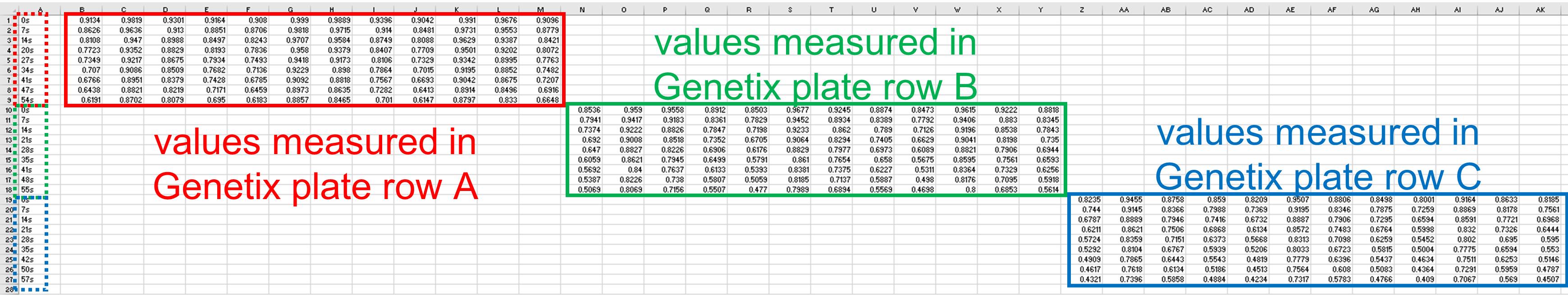
Figure 2. Example of raw data exported in Excel. Red, green and blue boxes show OD values measured in Genetix plate row A, B and C respectively. Red, green and blue dashed boxes show time stamps for Genetix plate row A, B and C respectively.Copy the values obtained from all measured rows of the Genetix plate into as many separated tabulated text files. To do this, you need to copy time stamps and monitored values for each plate row from the Excel sheet to a new tabulated text file (extension .txt). In these files, the first column must be time stamps in seconds, then OD values for columns 1–12 (or fewer). The first row is the header containing column names (could be numbers or specific names). During the 1 min monitoring, the plate reader can acquire 9–11 OD measurements, thus the text file should have 10–12 rows (including the column/sample names). An example of text file is provided in Table 1; it corresponds to the values obtained for a single plate row (row C in the provided dataset). At the end of this step, you should have as many text files as measured rows.
Table 1. Example of text file containing exported raw data. In this dataset, the plate reader measured nine points during 1 min acquisition; the first column contains time stamps in seconds and the first row contains column names. Here, samples are named from 1 to 12.
Time 1 2 3 4 5 6 7 8 9 10 11 12 0 0.8235 0.9455 0.8758 0.859 0.8209 0.9507 0.8806 0.8498 0.8001 0.9164 0.8633 0.8185 7 0.744 0.9145 0.8366 0.7988 0.7369 0.9195 0.8346 0.7875 0.7259 0.8869 0.8178 0.7561 14 0.6787 0.8889 0.7946 0.7416 0.6732 0.8887 0.7906 0.7295 0.6594 0.8591 0.7721 0.6968 21 0.6211 0.8621 0.7506 0.6868 0.6134 0.8572 0.7483 0.6764 0.5998 0.832 0.7326 0.6444 28 0.5724 0.8359 0.7151 0.6373 0.5668 0.8313 0.7098 0.6259 0.5452 0.802 0.695 0.595 35 0.5292 0.8104 0.6767 0.5939 0.5206 0.8033 0.6723 0.5815 0.5004 0.7775 0.6594 0.553 42 0.4909 0.7865 0.6443 0.5543 0.4819 0.7779 0.6396 0.5437 0.4634 0.7511 0.6253 0.5146 50 0.4617 0.7618 0.6134 0.5186 0.4513 0.7564 0.608 0.5083 0.4364 0.7291 0.5959 0.4787 57 0.4321 0.7396 0.5858 0.4884 0.4234 0.7317 0.5783 0.4766 0.409 0.7067 0.569 0.4507
Slope estimation on R
Open RStudio.
Create and save the script to analyze data in order to estimate the NADP-MDH activity defined as the initial slope and some other values (see Note 6).
Analyze data for the first text file:
Adapt line 3 in the script. You must type the name of text files between the quotation marks. As an example, if the text file name is rowC.txt, the line 3 should be: data_name="rowC.txt" (see Note 6).
Execute all the lines of the script. The script generates two outputs: a pdf file with curves of each monitored NADP-MDH activity, and a text file containing estimated slopes.
Open the pdf file and check every single curve. The curve should be bended or linear and continuously decreasing, without abrupt breaks. Example of expected curves and problematic curves are presented in Figure 3. Most unexpected shapes could be due to homogenization and/or bubble issues. It could be frequent at the beginning, but as soon as the gesture is mastered, it becomes rare.
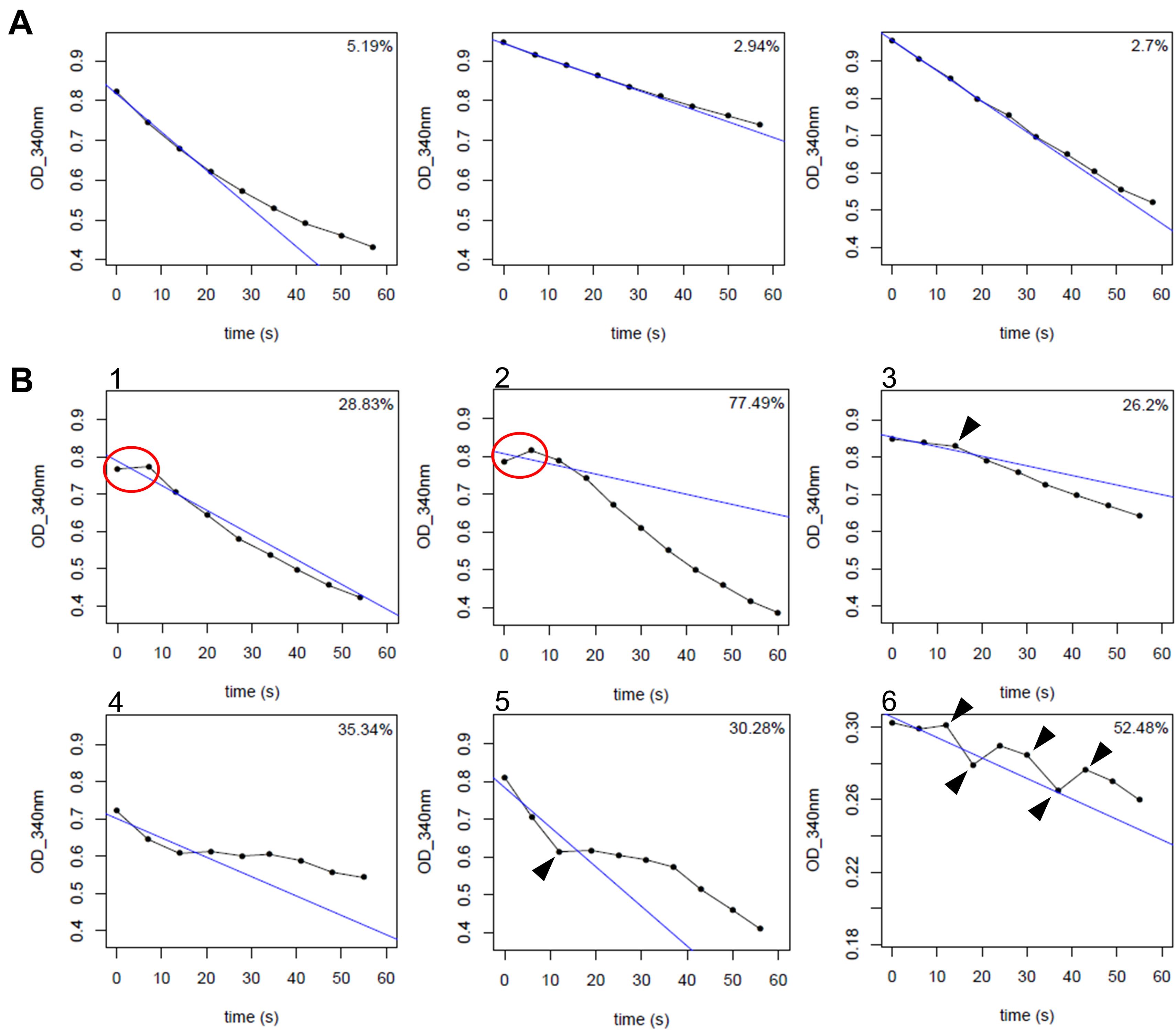
Figure 3. Example of NADP-MDH activity curves. Evolution of OD340nm over time showing the NADPH consumption by MDH. Blue line is the linear model calculated on the basis of the 4 first time points. Value printed in the top right corner is the coefficient of variation of the estimated slope. A. Example of expected curves. B. Example of problematic curves. Curves 1 and 2 have a first value lower than the second (indicated by circles). Curves 3, 5 and 6 have abrupt breaks (indicated by arrowheads).Check whether the calculated linear model correctly fits the curve or not. In addition to the curves’ quick check, we suggest using a criterion based on the slope coefficient of variation. We suggest discarding the slope value when this coefficient is higher than 15% (see Note 7).
Open the output text file. This file contains different values recorded for different curves: the estimated slope, its associated standard error calculated by the linear model, the coefficient of variation, and the calculated r of the linear model. An example of this output is presented in Table 2.
Table 2. Example of output text file. Extract of the output text file obtained with the dataset in Table 1. Slope: value of the estimated slope; coeffvar: value of the coefficient of variation; sd: calculated standard error of the slope value; rsquared: value of calculated linear model r.
rowC rowC_1 rowC_2 rowC_3 rowC_4 slope -0.00960714285714286 -0.00393999999999999 -0.00596571428571429 -0.00819714285714285 coeffvar 5.19414804028292000 2.94294762693293000 1.82244229793482000 1.48983689600294000 sd 0.00049900922244147 0.00011595213650116 0.00010872170051680 0.00012212405870378 rsquared 0.99463312400325000 0.99827080714040100 0.99933618176150200 0.99955627418466600
Proceed similarly for all text files.
Activity analysis for ex planta assay (alternative for D)
Calculate average initial activity and average maximal activity of the three measurements for each sample.
Calculate initial activity and maximal activity per microgram of protein.
Calculate activation ratio defined as the ratio of initial activity with maximal activity.
Perform statistical analysis using experimental replicates (see Note 8).
Activity analysis for in vitro analysis (alternative for C)
Plot activation kinetics with the calculated average activity.
Perform statistical analysis of experimental replicates (see Note 8).
Validation of protocol
This protocol was used to generate the data published by Baudry et al. (2022). The protocol reliability and reproducibility are illustrated in Figure 4 by a dataset row C, corresponding to raw data of NADP- MDH assays for four different samples of recombinant MDH performed in triplicate.
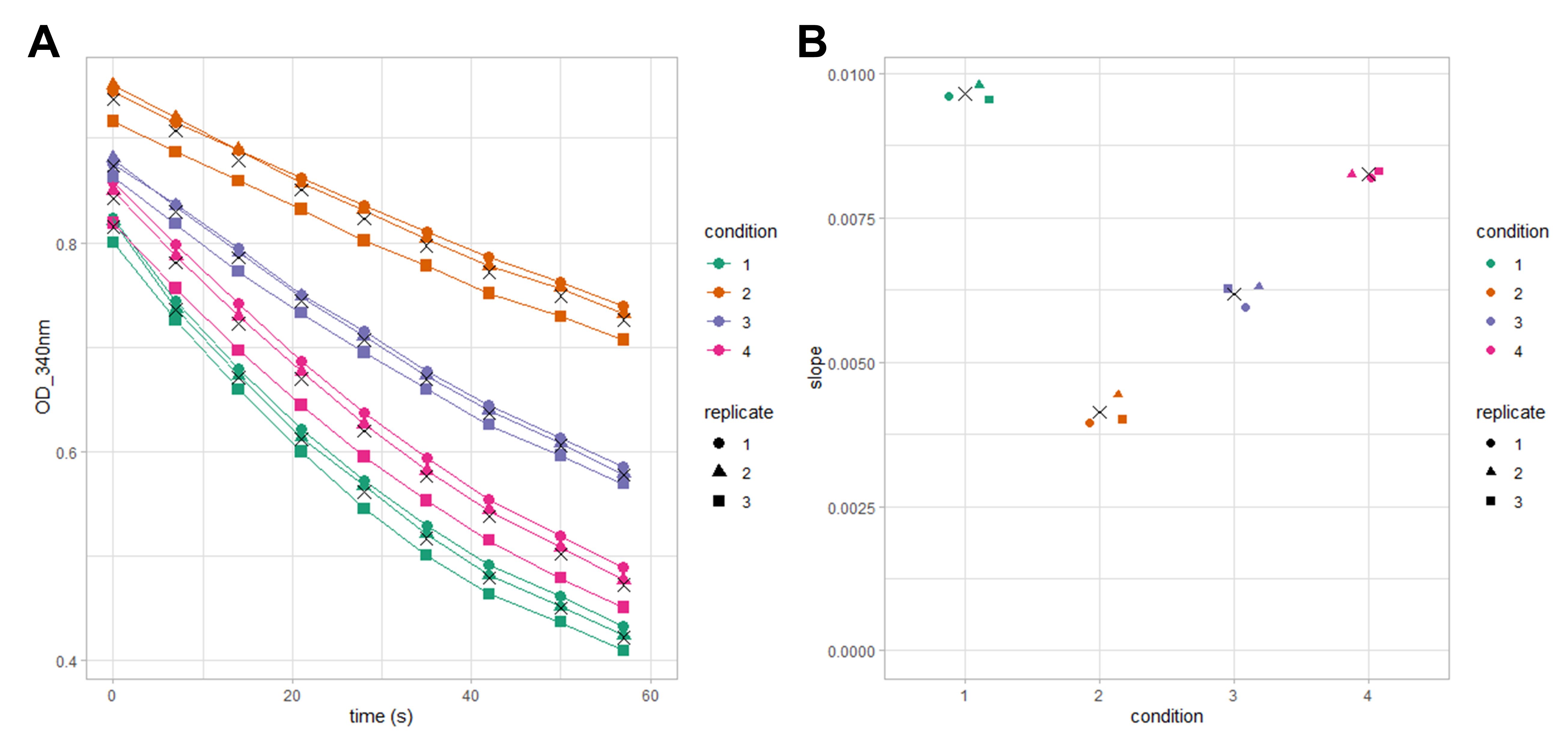
Figure 4. Example of replicate variation. NADPH consumption curves and deduced slope values obtained from three replicates of four different conditions, using recombinant MDH. A. NADPH consumption curves; symbols represent condition average values at each kinetics time point. B. Estimated slope absolute values of curves presented in A, symbols represent condition average values.
Notes
Protein quantitation can be performed using any other protein assay with a suitable range of sensitivity and using a standard spectrophotometer.
Leaf sampling: since NADP-MDH activation state undergoes fast variations with light intensity and along the light photoperiod, all leaf samples must be collected at the same time and in situ of plant culture. We recommend rapidly collecting leaves well exposed to the light and at the middle of the photoperiod. Leaf samples can be stored for several weeks at -80 °C after snap-freezing in liquid nitrogen.
M1 and M2 activation medium: recipes provided for M1 and M2 medium are standard conditions for full activation of NADP-MDH in vitro after 20 min incubation. This must be validated by checking that maximal activity has been obtained (activation plateau).
Tecan programming: to prewarm reaction medium and follow OD340nm for 1 min row by row, the Tecan must be programmed with its dedicated software Magellan. The programming is simple and consists in adding action boxes. The following program can be used for both types of assays. The user request function allows to pause the program until the user clicks on the pop-up, and allows to wait for the incubation times or during user actions:
Box Plate: select the type of plate.
Box Move Plate: check Out.
Box User Request: type a text to inform that user has to place the plate containing the reaction medium and prewarming is going to start.
Box Move Plate: check In.
Box Temperature: check On and set the temperature to 30.0 °C.
Box Wait for temperature: set minimum and maximum temperature to reach (recommendation: 29.5 and 31.0).
Box User Request: type a text to inform user that the temperature is reached.
Box User Request: type a text to inform user that Tecan is ready for measurement.
Box Move Plate: check Out.
Box User Request: type a text to inform user to mix sample in row A for measurement.
Box Move Plate: check In.
Box Part of Plate: select row A.
Box Kinetic Cycle: set Duration on 1 min.
Box Absorbance: set wavelength to 340 nm and number of flashes to 1.
Repeat steps 4h–4n for other plate rows (B to H).
Box Move Plate: check Out.
Recommendation to properly start NADP-MDH activity monitoring: using the multichannel pipette, quickly mix the sample with the assay medium. We strongly recommend mixing by stirring the mixture with the pipette tip making three or four turns. Do not mix by pipetting up and down to avoid making bubbles. Because the plate reader measures the OD vertically, bubbles can disrupt the measurement and make the data unusable. If bubbles form, you can try to quickly push them to the side; however, you run the risk of missing the complete row measurement by spending too much time on it, thus missing the beginning of the reaction. After mixing, as quickly as possible, hit the OK button on the software pop-up to move the plate in the plate reader and start monitoring.
R script to analyze raw data and calculate NADP-MDH activity: the following R script can be used to analyze data (plot curves of experimental data, slope estimation, coefficient of variation calculation, and export all these data as pdf and text files).
Line 3 (data_name="rowA.txt") must be adapted for every file to be analyzed.
Although not recommended, the window parameter (line 16) that defines which points are included in the linear model for the slope calculation can be modified for better fitting of some curves. In that case, the same parameter value should be used for all the samples (see Note 7).
<script>
##Data Import ####
#enter the data text file's name
data_name="rowA.txt"
#output file names creation
data_name.short=strsplit(data_name,split="\\.")[[1]][1]
pdf_name=paste0(data_name.short,".pdf") #output pdf name
outfile_name=paste0("Slope_",data_name.short,".txt") #output txt file name
#import raw data, change the column names and check that time stamp column is numeric
rawdata=read.table(data_name, header=T, sep="\t", check.names=F, comment.char="") colnames(rawdata)=c("time",paste(data_name.short,colnames(rawdata)[-1],sep="_"))
rawdata$time=as.numeric(gsub("s$","",as.character(rawdata$time)))
##Data Analysis ####
#parameters setting
window=c(1:4) #point used to estimate the slope, suggested default value = c(1:4)
MIN=min(rawdata[,-grep("time",colnames(rawdata))],na.rm=T) #lowest OD value, graphical parameter
MAX=max(rawdata[,-grep("time",colnames(rawdata))],na.rm=T) #highest OD value, graphical parameter
#slope estimation and plot
Slope.df=data.frame(matrix(nrow=4,ncol=ncol(rawdata)-1)) #data.frame to save slope estimation results
colnames(Slope.df)=colnames(rawdata[,-1])
row.names(Slope.df)=c("slope","coeffvar","sd","rsquared")
pdf(pdf_name) #export plots as a pdf
par(mfrow=c(3,4)) #12plots per page
for (i in 2:ncol(rawdata)) {
#slope estimation
LMtmp=lm(rawdata[window,i]~rawdata[window,"time"]) #estimation of the slope during the set window with a linear model
LMsum=summary(LMtmp)
Slope.df[c(1,3,4),(i-1)]=c(LMsum$coefficients[2,1:2],LMsum$r.squared) #save estimated slope, slope std error and the lm's r.squared
Slope.df[2,(i-1)]=100*abs(LMsum$coefficients[2,2]/LMsum$coefficients[2,1]) #coefficient of variation = sd/slope
#plot
plot(x=rawdata$time, y=rawdata[,i], ylim=c(MIN,MAX), xlim=c(0,60), pch=20, type="o", ylab="OD_340nm", xlab="time (s)", main=colnames(rawdata)[i]) #raw data plot
abline(LMtmp,col="blue") #plot the estimated slope
legend("topright","",bty="n",title=paste0(round(Slope.df[2,(i-1)],2),"%")) #add coefficient of variation value
#rm tmp data
rm(LMsum,LMtmp)
}
dev.off()
##Data Output ####
final.df=cbind.data.frame(data=rownames(Slope.df),Slope.df) #table to export as a txt file
colnames(final.df)[1]=data_name.short
write.table(final.df,outfile_name,row.names=F,col.names=T,quote=F,sep="\t") #print as a txt file a table containing the recorded slopes and others values
</script>
Slope coefficient of variation used: in this protocol, we define the measured NADP-MDH activity as the initial slope calculated on the basis of acquired data. For reliable results, the linear model used to estimate the slope should properly fit the curve. During the linear modeling, R estimates the intercept and the slope of the model and provides standard error value for both parameters. Our proposed coefficient of variation is the ratio of the slope standard error with the estimated slope value. We suggest discarding the slope value when this coefficient is higher than 15% to ensure reliability of the value. This value has been defined empirically, since most curves with a coefficient value higher than 20% (when the slope is calculated with four points) show an unexpected shape.
In Figure 3B, for five out of six example curves we might want to calculate the slope using only three points instead of four, as suggested. Removing the first time point cannot be considered for curves 1 and 2; since we try to measure the initial velocity, these curves should be discarded from the analysis. Removing the fourth point could be considered as long as all the slopes of the dataset are calculated on three points and the overall curve appearance is good (i.e., without an abrupt break). As an example, one can envisage doing such modeling on three points for curve 4 but not for curves 3 and 5. Curve 6 should be discarded from the dataset since it shows many break points.
According to the experimental design, different tests can be done. For example, for a design with one factor at two modalities (e.g., wild type vs. mutant), t-tests can be done; for one factor with more than two modalities (e.g., wild type, mutant 1, and mutant 2), one-way ANOVA should be done instead of t-test; for a design with more than one factor (e.g., wild type vs. mutant, both in mock and treatment conditions), a two-way (or more) ANOVA should be done. Although these tests cannot be done for kinetics, they can be done on calculated kinetic slopes, activity at a precise time point, etc.
Recipes
Following buffers, A, B, and C must be freshly prepared and kept on ice until used, since their oxidation could alter the results.
Extraction buffer for ex planta assay
100 mM Tris pH 6.8
Protease inhibitor cocktail for plant (diluted 100 times)
Activation medium for ex planta assay
50 mM DTT
50 μM recombinant TRX m type
Activation medium for the in vitro assay
The NADP-MDH activation mixture is as following: 0.24 μg/μL recombinant NADP-MDH; 10 mM DTT; 10 μM recombinant TRX m type; 30 mM Tris pH 7.9. To start the activation reaction, the two media M1 and M2 are mixed (by pipetting up and down three or four times) 1:1 vol:vol.
M1 contains only the NADP-MDH in Tris buffer:
0.48 μg/μL NADP-MDH
30 mM Tris pH 7.9
M2 contains all reagents, except NADP-MDH, in Tris buffer:
20 mM DTT
20 μM recombinant TRX m type
30 mM Tris pH 7.9
Reaction medium
160 μM NADPH
750 μM OAA
30 mM Tris pH 7.9
Prewarm at 30 °C.
This medium must be freshly prepared and cannot be stored more than half a day.
Acknowledgments
K.B. research was supported by a French Ph.D. fellowship from “Ministère de la Recherche et de l’Enseignement Supérieur.” IPS2 benefits from the support of the Labex Saclay Plant Sciences-SPS (ANR-17-EUR-0007). This protocol was used to produce the data published in the following research article: Baudry et al. (2022).
Competing interests
The authors declare no conflict of interest.
Ethics considerations
Any of these experimental procedures involved neither human nor animal subjects.
References
- Baudry, K., Barbut, F., Domenichini, S., Guillaumot, D., Thy, M. P., Vanacker, H., Majeran, W., Krieger-Liszkay, A., Issakidis-Bourguet, E., Lurin, C., et al. (2022). Adenylates regulate Arabidopsis plastidial thioredoxin activities through the binding of a CBS domain protein. Plant Physiol. 189(4): 2298–2314.
- Collin, V., Issakidis-Bourguet, E., Marchand, C., Hirasawa, M., Lancelin, J. M., Knaff, D. B. and Miginiac-Maslow, M. (2003). The Arabidopsis Plastidial Thioredoxins. J. Biol. Chem. 278(26): 23747–23752.
- Heyno, E., Innocenti, G., Lemaire, S. D., Issakidis-Bourguet, E. and Krieger-Liszkay, A. (2014). Putative role of the malate valve enzyme NADP–malate dehydrogenase in H2O2 signalling in Arabidopsis. Philos. Trans. R. Soc. Lond. B Biol. Sci. 369(1640): 20130228.
- Issakidis, E., Saarinen, M., Decottignies, P., Jacquot, J., Crétin, C., Gadal, P. and Miginiac-Maslow, M. (1994). Identification and characterization of the second regulatory disulfide bridge of recombinant sorghum leaf NADP-malate dehydrogenase. J. Biol. Chem. 269(5): 3511–3517.
- Jacquot, J. P., Issakidis, E., Decottignies, P., Lemaire, M. and Miginiac-Maslow, M. (1995). [25] Analysis and manipulation of target enzymes for thioredoxin control. In: Lester Packer (Ed.). Meth. Enzymol (pp. 240–252). Academic Press.
- Keryer, E., Collin, V., Lavergne, D., Lemaire, S. and Issakidis-Bourguet, E. (2004). Characterization of Arabidopsis Mutants for the Variable Subunit of Ferredoxin:thioredoxin Reductase. Photosynth. Res. 79(3): 265–274.
- Scheibe, R. (2004). Malate valves to balance cellular energy supply. Physiol. Plant. 120(1): 21–26.
- Scheibe, R. and Dietz, K. J. (2012). Reduction-oxidation network for flexible adjustment of cellular metabolism in photoautotrophic cells. Plant Cell Environ. 35(2): 202–216.
Article Information
Copyright
© 2023 The Author(s); This is an open access article under the CC BY-NC license (https://creativecommons.org/licenses/by-nc/4.0/).
How to cite
Baudry, K. and Issakidis-Bourguet, E. (2023). A Semi-throughput Procedure for Assaying Plant NADP-malate Dehydrogenase Activity Using a Plate Reader. Bio-protocol 13(16): e4769. DOI: 10.21769/BioProtoc.4769.
Category
Plant Science > Plant biochemistry > Protein
Biochemistry > Protein > Activity
Do you have any questions about this protocol?
Post your question to gather feedback from the community. We will also invite the authors of this article to respond.
![]() Tips for asking effective questions
Tips for asking effective questions
+ Description
Write a detailed description. Include all information that will help others answer your question including experimental processes, conditions, and relevant images.